ECE 1230 F26 U3 L6 S Domain Analysis
Overview
Angela Rasmussen introduces S-domain circuit analysis as a way to replace differential-equation work with impedance-based algebra for arbitrary inputs, using R, sL, and 1/(sC) when initial conditions are zero. She demonstrates unit-step notation, nodal analysis, transfer functions, and how characteristic roots indicate damping, oscillation, and stability, with MATLAB as a tool for solving more complicated equations.
Key takeaways
- For zero-initial-condition RLC analysis, replace jω with s: resistors stay R, inductors become sL, and capacitors become 1/(sC).
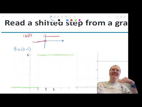
- A delayed step that turns on at t = a is u(t − a); scaling it by A models a signal of amplitude A that begins at that time.
- A transfer function is the S-domain output divided by the input, and it describes how a circuit responds across frequencies.
- Characteristic roots distinguish common second-order responses: distinct real roots are overdamped, repeated real roots are critically damped, and complex roots are underdamped.
- For a stable circuit, characteristic roots must have negative real parts; their real components set decay rates and their imaginary components set oscillation rates.
- MATLAB can solve simultaneous nodal equations and find roots for higher-order circuits, avoiding lengthy hand calculations.
Chapters
- The lecture moves beyond phasors, which assume a single sinusoidal frequency, toward analyzing inputs with arbitrary waveforms.
- Fourier series and the Fourier transform are mentioned as ways to represent signals as combinations of sinusoids.
- The Friday quiz covers phasor-based Thévenin equivalents; MATLAB is recommended for the required solution, with a screenshot of the work.
- The basic conversion replaces jω with s, yielding the S-domain model for RLC circuits.
- The method introduced here assumes zero initial conditions for capacitors and inductors.
- Nonzero initial conditions require additional source terms in the element models, which the lecture does not develop.
- The unit step u(t) is zero for t < 0 and one for t ≥ 0, representing power being connected at time zero.
- The step function gives a mathematical model for a switch that changes the circuit state at a specified instant.
- Its graph marks the value at t = 0 as filled, while values before zero remain zero.
- A step delayed until t = 1 is written u(t − 1); multiplying it by 5 gives a step of amplitude 5.
- The shift is chosen so the step argument equals zero at the switching time, such as t = 1 for u(t − 1).
- A constant or sinusoidal signal can be multiplied by a shifted unit step to keep it off until the specified time.
- The graph exercises translate constant levels such as 3 and −2 into 3u(t) and −2u(t).
- A signal that becomes −4 at t = 5 is represented by −4u(t − 5), not a positively shifted step.
- The examples distinguish signal amplitude from switching time and apply the same step gate to a sinusoidal input.
- Frequency domain is the broad term; phasor analysis typically specifies one angular frequency, while S-domain analysis uses the Laplace variable s.
- Impedance methods replace differential equations and repeated integration with algebraic circuit equations.
- Frequency response helps identify operating bands relevant to Wi-Fi, aviation, medical devices, audio filters, and noise rejection.
- Replacing jω with s gives an inductor impedance of sL and a capacitor impedance of 1/(sC); resistance remains R.
- Although written without j, s is a complex variable, and the impedances retain units of ohms.
- A Laplace transform table pairs u(t) with 1/s; the lecture uses such transform results without deriving them.
- For nonzero initial conditions, extra terms are needed; the examples use zero initial conditions and the simpler element impedances.
- The worked circuit replaces its source with a variable V(s), leaves resistors unchanged, and converts the 3 mH inductor to 3 × 10⁻³s.
- The 50 μF capacitor becomes 1/(50 × 10⁻⁶s), while the 3 Ω resistors remain 3 Ω.
- After choosing ground and labeling nodes, branch currents are written as node-voltage differences divided by their S-domain impedances.
- Kirchhoff's current law produces simultaneous equations in V₁ and V₂, with parentheses needed to preserve factors such as 50 × 10⁻⁶s.
- Solving the nodal equations for V₂ expresses the output as a function of s multiplied by the input V(s).
- Dividing output by input gives the transfer function, a compact description of circuit response.
- The example circuit is a notch filter: it passes frequencies on either side of a rejected frequency and suppresses the output at the notch.
- Time-domain examples show the output sinusoid shrinking near the notch frequency and disappearing at the rejection point.
- The S-domain characteristic polynomial avoids directly solving high-order differential equations; MATLAB can help find its roots.
- For a second-order polynomial, a positive discriminant gives distinct real roots, zero gives a repeated root, and a negative discriminant gives complex roots.
- Distinct real roots correspond to overdamped behavior, repeated real roots to critical damping, and complex roots to underdamped oscillation.
- Damping choices affect settling behavior: critical damping settles without oscillation, while underdamped responses can overshoot and oscillate.
- A practice circuit is converted to S-domain impedances before writing its current as a sum of branch currents.
- For the example, the input-current-to-voltage expression includes the conductance terms 1/10, 2s, and 3/s.
- The expression can be used to find characteristic roots and determine whether the system has real or complex poles.
- Pole-zero plots use x marks for poles and circles for zeros; stable-system poles lie in the left half of the complex plane.
- The second worked circuit converts its inductor to 2s and its capacitor to 3/s, while retaining the resistor value.
- Nodal analysis labels the unknown node voltage Vx and writes branch currents using impedances 10, 2s, and 3/s.
- Because the capacitor voltage is measured from Vx to ground, Vc = Vx; solving the node equation gives the requested output.
- Combining the equation into a polynomial allows its roots to be inspected, though the expected exam work is primarily the S-domain expression.
- A further circuit example targets removal of low- and high-frequency noise and asks for the inductor current.
- The source and resistor values remain unchanged in the S-domain conversion, while the capacitor and inductor become functions of s.
- The node voltage is found by Kirchhoff's current law using the capacitor branch impedance 3/s and the inductor-resistor branch impedance 20 + 2s.
- The inductor current follows from the voltage across its branch; the resulting roots indicate damping behavior.
- Real parts of roots determine exponential growth or decay rates, while imaginary parts determine oscillation frequency.
- For a stable circuit, roots should have negative real parts and lie in the left half of the complex plane.
- A step response describes how a system reacts when its input changes from no power to power, including a processor load changing from idle to full load.
- Power-converter filters use response analysis to limit voltage droop when load current changes.
- The lecture closes with a reflection on which S-domain concepts may need further practice.
- Students are reminded to complete the required professional activities and attend one seminar; the announced seminar begins at 3:00.
- Angela Rasmussen notes that participation-grade import errors should be reported and that reflections can be submitted for extra credit.
- The next class sessions will extend the method to more complicated circuits with additional sources and elements.
Transcript excerpt
0:08 Okay. Hi, welcome. Is it going to stay? Okay. I think it's gonna stay. All right. So, today we're going to talk about the movement. So, we've been doing the phasers. Um, and now we're going to move to where you don't know what the input might be. And so we have any input. We don't know what omega is. So what do we do as far as transforming those circuits into the s domain. So this is nice because it allows us to look at any input signal. It doesn't have to be a very specific sinosoid. It can be any signal. Um which makes it kind of nice. Um and it doesn't have to be one just one frequency. [clears throat]
0:55 So a lot of times signals may be a combination of a whole bunch of of sinosoids. So as you move forward in your classwork in 3500, you're going to learn how to actually look at any signal and mathematically express it in terms of a whole bunch of summations of sinosoids, which is a powerful thing that can be done. And so any signal can be um a whole bunch of other signals and so they can be different frequencies. They can be different amplitudes and you can express any arbitrary signal by that which is really cool. It's called the forier. There's a forier series which is the summation of all those together. But then there's the forier transform which is when you use that technique to move
1:42 into the frequency domain. What we're going to focus on today is what's called the S domain. And so, um, I guess before I move on, so make sure you take the quiz. It's due by Friday. And I think last time I did mistakenly say what it was going to be on. It's
This is the start of the transcript. Save this video free for the whole transcript, searchable and time-coded.
Related notes
Summary, takeaways, and chapters were generated by AI from the video's transcript and may contain errors. The video belongs to its creator, University of Utah: Professor Angela Rasmussen.