ECE 1230 F26 U3 L4 Phasor Domain Analysis Examples
Overview
Angela Rasmussen teaches a complete workflow for AC circuit analysis in the phasor domain: convert sources and R, L, and C components, write complex KCL equations at extraordinary nodes, solve for phasors, and interpret or transform results back to the time domain. Worked examples use a 35 rad/s circuit and a two-node network, with MATLAB as a solver and quadrant checks to catch phase errors; the lecture also connects impedance phase to leading and lagging and to resistor-inductor behavior.
Key takeaways
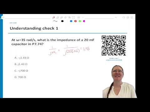
- In the phasor domain, use R unchanged, replace an inductor with jωL, and replace a capacitor with 1/(jωC); at ω = 35 rad/s, a 20 mF capacitor is -1.43j Ω.
- Write complex KCL by identifying extraordinary nodes and expressing each branch current as its voltage difference divided by impedance; do not include open paths that carry zero current.
- Use rectangular form to add or subtract complex quantities and polar form to interpret magnitude and phase; verify each angle against the quadrant implied by the real and imaginary signs.
- A negative imaginary impedance sign indicates phase direction, not a smaller magnitude; capacitors have negative imaginary impedance and inductors have positive imaginary impedance.
- Voltage and current phase differences reveal circuit behavior: current at -30° relative to voltage at 0° lags, and their ratio gives an impedance with +30° phase, consistent with resistance and inductance.
- MATLAB can solve simultaneous complex KCL equations, but correct parentheses and explicit degree units matter; check solver output against hand-derived equations and quadrant expectations.
Chapters
- The week’s quiz asks students to analyze a circuit whose time-to-frequency conversions are already provided.
- The target workflow is to solve the phasor-domain circuit and interpret its output, rather than repeat the conversions.
- Resistors remain R, inductors become jωL, and capacitors become 1/(jωC).
- For an inverse phasor transform, use the magnitude as the cosine amplitude, the phasor angle as phase, and the original signal’s ω in the cosine argument.
- Complex KCL requires identifying extraordinary nodes, defining branch currents, and excluding open paths with zero current.
- Rasmussen recommends Unit 3 practice problems, past exams, the Ulaby textbook, and starred end-of-chapter problems.
- AC sources are physical voltage or current inputs; a voltage source commonly drives current through circuit components.
- A transistor can act as a voltage-controlled current source, a topic students encounter in ECE 2280.
- For C = 20 mF and ω = 35 rad/s, the capacitor impedance magnitude is about 1.43 Ω.
- Since 1/j = -j, the impedance is -1.43j Ω; the negative imaginary sign is essential.
- Angular frequency defaults to radians per second unless the problem specifies another unit, such as hertz.
- The example uses ω = 35 rad/s and an input current phasor of 18∠75°.
- The 20 mF capacitor becomes -1.43j Ω, while 80 mH and 30 mH inductors become 2.8j Ω and 1.05j Ω.
- After replacing the reactive components, the remaining task is to write node equations and solve for the requested current.
- At node V1, write each branch current using its voltage difference divided by impedance, including V1/(2.8j) for the inductor branch.
- The current source 18∠75° enters the node; the resistor-capacitor and resistor-inductor branches carry currents based on their respective impedances.
- The computed output is approximately 2.06∠153°; use the original 35 rad/s to express the result in the time domain.
- At extraordinary node V1, Rasmussen writes outgoing currents as V1/(50 - 1.43j), V1/(2.8j), and V1/(24 + 1.05j), with 18∠75° entering.
- In MATLAB, use j for the imaginary unit and parentheses around complex denominators and numerators to preserve the intended equation.
- Specify 75 degrees explicitly when entering the source; otherwise a tool may interpret the angle in radians.
- The MATLAB result for the example current is 2.06 at 153°, which maps to a 2.06-amplitude cosine with the original 35 rad/s frequency.
- An exam may expect students to set up expressions and interpret results, with arithmetic simple enough to do by hand rather than requiring MATLAB.
- A negative imaginary sign changes the phasor’s direction, not its magnitude; among the listed reactive impedances, 1.05 Ω is the smallest magnitude.
- A phasor in quadrant II should have an angle between 90° and 180°; the example’s 153° result fits that check.
- The sign of real and imaginary components determines the quadrant, so a negative value is not automatically a smaller impedance or current.
- Rasmussen connects phase accuracy to practical power systems, noting that incorrect phase handling in grid inverters can misdirect power and damage equipment.
- The next example begins with components already converted to frequency-domain impedances, focusing practice on equations rather than conversion.
- Students identify V1 and V2 as extraordinary nodes and write branch currents from node-voltage differences.
- Rasmussen encourages checking answers against expected quadrants and using MATLAB or another verified solver for the simultaneous complex equations.
- For the V1-to-ground branch, the current is V1/(6 - 4j); the branch between nodes carries (V1 - V2)/(12j).
- The V1 KCL has source currents 2 and 4 entering, balanced by the two outgoing branch currents.
- The V2 KCL includes the inter-node current, an entering -3j source, and outgoing terms 4 and V2/(6 - 4j).
- Parentheses around V1, V2, and complex impedances are necessary when entering the equations in MATLAB.
- Rasmussen corrects a copied answer: V1 = 20.7 + 16.1j and V2 = -20.7 - 42.1j in rectangular form.
- V1 lies in quadrant I and has an angle near 37.8°; V2 lies in quadrant III and has an angle near -116°.
- A time-domain expression cannot be recovered without the input signal frequency, even when the node-voltage phasors are known.
- For V2 = -20.7 - 42.1j, quadrant III rules out candidate angles such as +116°, -64°, and -42°; an angle near -116° is consistent.
- Comparing a voltage phasor at 0° with a current phasor at -30° shows that the current lags the voltage.
- Dividing voltage by current gives an impedance magnitude of 4 and a phase of +30°, identifying a positive real and positive imaginary combination.
- A positive real impedance component corresponds to a resistor, while a positive imaginary component corresponds to an inductor; a 4∠30° impedance therefore indicates R-L behavior.
- Students are asked to identify weak points and practice the specific steps that need more work, including conversion, KCL setup, solving, and phase interpretation.
- Rasmussen suggests MATLAB and course problem sets for practice, and mentions Google Gemini’s notebook feature for generating concept quizzes from uploaded notes.
Transcript excerpt
0:03 All right, so welcome. Um, again, if you are not physically here, make sure you're taking the attendance quiz and then for everyone, there's going to be a quiz this that's due by this Friday night. And it will be an analysis where where you'll be given, you know, such a circuit as this, and you'll need to do um since you already did the conversions in the last one, the conversions will already be done, but you'll need to make sure that you can solve this kind of a circuit in that frequency domain. Okay? So that's the goal of this week is that you are able to analyze this in that frequency phasor
0:53 estimate. So that will be due required by Friday night, so make sure that you do complete that. [snorts] All right, so we've talked about this multiple times, but we are able now to convert from time domain into the frequency domain by doing these phasor transforms. So we can take a signal, transform them as phasor transform and go from cosine into a polar form. Each of the components for an inductor, how do we transform into the frequency domain? Anyone?
1:54 So if we have the inductor, transforming it into the frequency domain, What's the equation? For the capacitor, what's the expression for those conversions? >> J omega L. >> Thank you. >> And then one over J omega C. >> Great. Yes. So and then what happens to R?
2:45 Correct. So R just stays the same. So you don't have to do anything with R, just rewrite it. Ls you have to do J omega L. Cs you have to do one over J omega C. Where does that omega come from? Correct. So from this one is where those omegas come from.
This is the start of the transcript. Save this video free for the whole transcript, searchable and time-coded.
Related notes
Summary, takeaways, and chapters were generated by AI from the video's transcript and may contain errors. The video belongs to its creator, University of Utah: Professor Angela Rasmussen.