ECE 1230 F26 U3 L3 Phasor Domain Analysis
Overview
Professor Angela Rasmussen teaches ECE 1230 students to analyze sinusoidal circuits by converting components and sources to the phasor domain, writing node-voltage KCL equations, and solving the resulting complex system with MATLAB or a calculator. She also introduces dependent sources and small-signal transistor models, then applies impedance methods to find Thevenin voltage and impedance, including a worked example with Zth = 50 - 43.24j ohms.
Key takeaways
- Convert sinusoidal circuit elements to impedances before writing node equations: resistors stay unchanged, inductors become jωL, and capacitors become 1/(jωC).
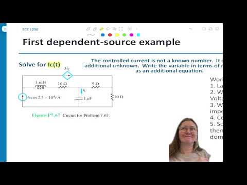
- Dependent sources require an explicit equation relating the controlling variable to circuit quantities; in the worked example, Ic must be defined from the capacitor branch voltage and impedance to complete the equation system.
- For complex arithmetic, use rectangular form for addition and subtraction and polar form for multiplication and division, then convert solved phasors back using the original angular frequency.
- An independent-source Thevenin impedance is found by shorting ideal voltage sources and opening ideal current sources, then reducing the impedance seen at the output terminals.
- A negative imaginary impedance denotes capacitive behavior, while a positive imaginary impedance denotes inductive behavior; the example’s 50 - 43.24j Ω therefore contains resistive and capacitive components.
- When finding Thevenin impedance with dependent sources, keep dependent sources active and use a test source, with ZTH = Vtest/Itest.
Chapters
- The week’s AC quiz asks students to set up and solve node-voltage equations after converting a circuit to the frequency domain.
- MATLAB is recommended for solving complex systems; Rasmussen cautions that Wolfram Alpha and general-purpose AI tools are not vetted for reliable answers.
- Professional career engagement activities are due by the end of the semester.
- A diamond marks a dependent source; plus/minus indicates a dependent voltage source, while an arrow indicates a dependent current source.
- Examples include a voltage source of 5Vx or 3I1 and a current source of 2I2 or a value controlled by Vx.
- The controlling variable must be defined and labeled elsewhere in the circuit.
- Coefficients carry units that make the source expression correct: a current-controlled voltage source uses ohms, while a voltage-controlled current source uses siemens.
- Resistors, capacitors, and inductors are treated as linear elements, while diodes and transistors have nonlinear behavior outside their operating region.
- A small-signal transistor model represents behavior in a linear operating region using simple circuit elements, including dependent sources.
- The four dependent-source types are VCVS, CCVS, CCCS, and VCCS, classified by whether voltage or current controls voltage or current.
- Circuit analysis supports design, but simulation and physical testing remain important checks on whether a circuit works in practice.
- The worked circuit’s target is capacitor current Ic, which also controls a dependent current source labeled 3Ic.
- Because the circuit includes multiple energy-storage components, the full circuit is converted to the frequency domain before solving.
- The analysis begins by locating the requested variable and identifying where it appears both as an output and as a controlling quantity.
- A zero-phase sinusoidal source such as 6e^j0 becomes the real phasor 6.
- Inductor impedance is ZL = jωL, and capacitor impedance is ZC = 1/(jωC).
- For the example’s angular frequency of 25,000 rad/s, Rasmussen demonstrates substituting ω and component values into the impedance formulas.
- Resistors retain their resistance values in the phasor domain; reactive components become complex impedances in ohms.
- The circuit is organized around three extraordinary nodes, labeled V1, V2, and V3, with the bottom node selected as ground.
- A current is assigned to each branch between extraordinary nodes; arbitrary directions are valid if used consistently.
- Known current-source directions are followed, and the dependent branch is labeled Ic.
- Branch currents are written using node-voltage differences divided by complex impedance, just as with resistors.
- At V1, the 6 A source supplies the outgoing dependent-source current 3Ic and the current through the branch between V1 and V2.
- At V2 and V3, KCL uses the corresponding node-voltage differences across the complex impedances and resistors.
- A fourth independent relation is needed for the target current, defined directly from its branch voltage and impedance, such as Ic = V2/ZC.
- Using a relation already embedded in another KCL equation does not provide the required additional independent equation.
- MATLAB can solve the simultaneous complex equations for V1, V2, V3, and Ic; calculators with complex-system capability are alternatives.
- Check results by substituting the solved values into the original equations and confirming both sides match.
- Convert the solved current phasor to polar form, then use its magnitude and phase in the time-domain cosine at the original angular frequency.
- The solved node phasors can also be converted back to time-domain voltages.
- Thevenin analysis in the frequency domain finds open-circuit voltage VTH and complex impedance ZTH.
- VTH is the voltage difference between output terminals A and B; ZTH is the impedance seen looking into those terminals.
- For independent sources, suppress voltage sources as shorts and current sources as opens when finding ZTH.
- Use rectangular form for addition and subtraction, and polar form for multiplication and division.
- The source frequency sets ω = 40,000 rad/s for the example circuit.
- A 1 mH inductor becomes 40j ohms, and a 0.5 μF capacitor becomes -50j ohms.
- The 25 Ω, 35 Ω, and 350/37 Ω resistors remain unchanged in the phasor circuit.
- The source is converted to its phasor before separate circuits are analyzed for VTH and ZTH.
- The output voltage is measured between A and B, with B chosen as ground in the worked example.
- The circuit has one extraordinary node, V1; a branch ending at an open output carries no current and therefore does not create another independent node voltage.
- VTH can be found by treating the output voltage as a node voltage or by using Ohm’s law to calculate the drop across the output resistor.
- The 3 A source remains active while calculating open-circuit voltage.
- The branch currents are expressed with the complex impedances 40j + 25 Ω and 35 - 50j Ω.
- KCL at V1 equates the incoming current through the 40j + 25 Ω branch and the 3 A source to the outgoing current through 35 - 50j Ω.
- After solving for V1, the output voltage is calculated from the current through the 35 - 50j Ω branch and the -50j Ω output impedance.
- MATLAB’s solve function or a complex-capable calculator can handle the resulting equations.
- For ZTH, the 3 A independent current source is opened, and the output terminals are used to trace the remaining impedance paths.
- The 350/37 Ω branch is in series with a parallel combination of -50j Ω and 60 + 40j Ω.
- The resulting Thevenin impedance is 50 - 43.24j Ω.
- The positive real part represents a 50 Ω resistor; the negative imaginary part indicates capacitive reactance.
- A quick check at ω = 40,000 rad/s gives 40j Ω for a 1 mH inductor and -50j Ω for a 0.5 μF capacitor.
- Students then work a second circuit using a 4 mH inductor, an 80 μF capacitor, and resistors.
- The second circuit’s sources are 12cos(2500t) V and 0.5cos(2500t - 30°) A, so their phasors use ω = 2,500 rad/s.
- At that frequency, the inductor and capacitor impedances are 10j Ω and -5j Ω, respectively.
- The known 12 V source node is used directly, alongside extraordinary nodes V1 and V2.
- The branch currents include (12 - V1)/10, V1/(-5j), (V1 - V2)/(10j), the 0.5∠-30° A source, and V2/10.
- KCL at V1 and V2 yields the node voltages; because B is ground, VTH equals V2.
- The worked result is reported as VTH = -12 V, a negative real phasor relative to the chosen reference.
- To find ZTH, the 12 V source is replaced by a wire and the independent current source by an open circuit.
- The reduction combines 10j Ω in parallel with -5j Ω, then places that result in the indicated parallel network with 5 Ω and 10 Ω branches.
- The reactive contributions cancel in the final reduction, producing the reported ZTH = 0 Ω.
- With dependent sources present, suppress only independent sources, retain the dependent source, apply a test source, and calculate ZTH = Vtest/Itest; VTH is found as usual.
Transcript excerpt
0:03 All right, welcome. Hopefully everybody had a great week great fall weekend. Um, couple things. If you are not here and you guys are watching this online, make sure you're taking the attendance um quiz as a substitute for you guys that are here. We'll do a poll everywhere to take your attendance. Um, quiz is due by Friday. It's going to be an AC uh phasor analysis. So I will last Friday was to test that you could convert the components into the frequency domain. So now this next step is once it's transferred into the frequency domain, being able to set up the set of
0:50 equations and being able to solve for those. So that is what the focus of this week's is going to be is setting up the node voltage expressions and being able to solve for them. So again, you'll be able to use MATLAB um MATLAB to be able to do that. Again, Wolfram Alpha is not showing to be correct for some reason, so I would not suggest that one. Chat GPT, Claude, any of the others also are not vetted tools that that have been proven beyond anything that they're always correct. So don't rely on those either. All right, any questions about the material up to this date? Any questions about the course? Also another reminder, if you haven't done your professional career
1:39 kind of engagement activities, make sure that you're also doing those. They will be due by the end of the semester. Okay. So last time we went through how to convert and then we also did a review on conversion and then we also learned on how to set up the complex expressions for the voltage expressions. So, one thing is that we haven't talked about a lot, but
This is the start of the transcript. Save this video free for the whole transcript, searchable and time-coded.
Related notes
Summary, takeaways, and chapters were generated by AI from the video's transcript and may contain errors. The video belongs to its creator, University of Utah: Professor Angela Rasmussen.