*CE 312 Lecture 18: Shear/Moment Diagrams III, Distributed Loads (2026.09.28)
 Watch on YouTube →
Overview
Gregory Michaelson explains how to construct shear and moment diagrams for distributed loads using the relationships between load, shear, and moment: constant loads produce linear shear diagrams, and linear shear produces quadratic moment diagrams. A worked beam example calculates reactions of 80 kips at A and 190 kips at C, then uses shear-diagram areas to obtain moment values and identify the diagram’s shape.
Key takeaways
- For a constant distributed load, shear changes linearly at a rate equal to the load intensity; integrating that linear shear produces a quadratic moment curve.
- A distributed load may be replaced by a single resultant to calculate support reactions, but the original load distribution must be retained when constructing shear and moment diagrams.
- The beam example’s reactions are 80 kips upward at A and 190 kips upward at C; its shear sequence is +80, -40, -70, -130, +60, then zero.
- The moment at a location is found by accumulating signed areas under the shear diagram; the example reaches +1,066.67 foot-kips at the zero-shear point and -1,200 at C.
- A point load creates a sudden shear jump and therefore an abrupt change in moment-diagram slope, while the moment itself remains continuous at the load location.
Chapters
- Homework 5.1 solutions will be posted, Homework 5.2 is due, and Homework 5.3 is assigned for the next lecture.
- Michaelson recommends installing MASTAN2 before a later assignment and having laptops ready for upcoming Microsoft Excel work.
- The lecture applies shear and moment diagram methods to distributed loads after earlier work with concentrated loads.
- Integrating a constant distributed load produces a linear shear diagram.
- Integrating linear shear produces a quadratic, parabolic moment diagram.
- A change in shear magnitude indicates a change in the moment diagram’s slope, described as moving from a lot of slope to a little or the reverse.
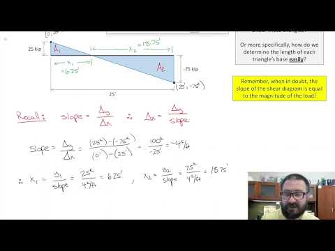
- For a shear line falling from +25 kips to -75 kips over 25 feet, the slope is -4 kips per foot.
- The triangle widths are 6.25 feet for the +25-kip portion and 18.75 feet for the -75-kip portion.
- Using one-half base times height gives areas of +78.125 and -703.125 foot-kips; the widths check because they sum to 25 feet.
- The beam has supports at A and C, a 3-kip-per-foot load over 60 feet, a 30-kip point load at 40 feet, and a 60-kip load at the 80-foot endpoint.
- For reaction calculations, Michaelson replaces the distributed load with its 180-kip resultant acting 30 feet from A.
- Summing moments about A gives C_y = 190 kips upward; vertical force equilibrium then gives A_y = 80 kips upward, and A_x = 0.
- The 180-kip equivalent load is only for calculating support reactions; using it to construct the moment diagram would misrepresent the distributed loading.
- Starting at A, shear jumps to +80 kips, falls linearly by 120 kips to -40 at B, then drops 30 kips to -70.
- Across B to C, the 3-kip-per-foot load reduces shear by 60 kips to -130; the 190-kip reaction at C raises it to +60.
- Shear stays at +60 from C to D before the 60-kip endpoint load returns it to zero, checking vertical-force equilibrium.
- The C-to-D shear rectangle has area 60 kips times 20 feet, or +1,200 foot-kips.
- The B-to-C trapezoid averages shear values of -70 and -130 kips over 20 feet, giving -2,000 foot-kips.
- On A-to-B, the -3-kip-per-foot shear slope places the zero crossing 26.67 feet from A, leaving 13.33 feet to B.
- The A-to-B triangle areas are +1,066.67 and -266.67 foot-kips, placing the moment at B at +800 foot-kips and confirming the area balance.
- Moment starts at zero at A, reaches a maximum of +1,066.67 foot-kips where shear crosses zero, and falls to +800 at B.
- The B-to-C shear area reduces moment by 2,000 foot-kips to -1,200 at C; the C-to-D rectangle raises it back to zero at D.
- The moment curve is parabolic under the distributed load from A to B and from B to C, then linear from C to D where shear is constant.
- The 30-kip point load at B causes shear to jump from -40 to -70, so the moment slope changes abruptly and separate parabolas meet at B.
Transcript excerpt
0:04 Okay, so this is lecture 18 in structural analysis. Uh, so just a couple of housekeeping items since I'm pre-recording this uh for my uh trip next week. Um, I don't know where the uh status of the homework is. Uh, but I'm guessing my my uh TA is going to largely keep up to date with it. Um, one thing I'll say is by the time this lecture goes live, homework 5.1 solution will be posted. Homework 5.2 2 will be uh due at the time this lectures uh goes live and then homework uh 5.3 will be assigned today at 11:00 a.m. due the following lecture. Um since this is going to be the first of a series of pre-recorded lectures, I did want to mention something for this week. Um number one, um this uh at least for for the next lecture, I would try and have your laptops ready when you watch that because we're going to be doing some
0:51 Microsoft Excel work uh for for the next lecture. The other thing I wanted to mention for this week, since we're going to be uh doing this sort of at a distance, is this would be a great time to go ahead and install Mass Tan 2 on your machine. It's both Windows and Mac friendly. And I think um that uh this would be a good day to sort of work out the kinks and whatnot. There's an assignment a little bit later where you have to post um proof that you did it. Um and we do that prior to actually using it in class. So, everybody will get it installed, but it would just be kind of a nice idea to go ahead and do that now. Uh, okay. So, let's go ahead
This is the start of the transcript. Save this video free for the whole transcript, searchable and time-coded.
Related notes
Summary, takeaways, and chapters were generated by AI from the video's transcript and may contain errors. The video belongs to its creator, Gregory Michaelson.