10:3 Pipe Flow - Major Losses, Minor Losses, Type I and II Systems
Overview
Derek Elsworth explains how to combine Darcy–Weisbach major losses, fitting and valve minor losses, and the energy equation to calculate pipe-system head requirements. He applies momentum and energy balances to a 100 kg person lifted by a jet-powered water system, estimating a 10 m/s jet, about 16 m of pump head, and roughly 16 kW of power, then previews Type I, II, and III pipe-flow problems.
Key takeaways
- Major pipe loss is calculated with Darcy–Weisbach, hL = f(L/D)(V²/2g), while each fitting or transition adds a minor loss of K(V²/2g).
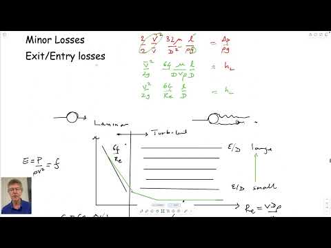
- The Moody chart links friction factor to Reynolds number and relative roughness: laminar flow uses f = 64/Re, while fully rough turbulent flow is nearly independent of Reynolds number.
- A loss coefficient near 1 for a pipe exit into a large tank reflects dissipation of nearly all the incoming velocity head as the fluid comes to rest.
- In the jet-lift estimate, a 100 kg load and a 0.01 m² water outlet imply a jet velocity of about 10 m/s from the momentum balance.
- The example’s 10 m/s flow, 10 m pipe, 0.1 m diameter, and fitting losses yield an estimated pump head of about 16 m and hydraulic power of about 16 kW.
- Known flow makes a Type I pipe problem direct; pressure-drop problems and pipe-sizing problems require estimating or iterating on velocity and friction factor.
Chapters
- A jet-powered water-flight clip introduces the example Elsworth uses to connect pipe flow with conservation of momentum.
- A US pipeline map distinguishes natural-gas transmission routes, hazardous-liquid pipelines, and underground gas storage.
- The map shows a trunk line serving State College, including a connection to a local heating plant.
- The Darcy–Weisbach major-loss relation is hL = f(L/D)(V²/2g), using average pipe velocity.
- For laminar flow, the friction factor is f = 64/Re; turbulent-flow friction depends on relative roughness and, in some regimes, Reynolds number.
- In fully rough turbulent flow, the Moody-chart friction factor becomes nearly independent of Reynolds number.
- The energy equation balances elevation, pressure head, velocity head, pump head, and head loss between upstream and downstream locations.
- Major losses represent wall friction and scale with f(L/D)(V²/2g).
- Minor losses represent fittings and flow transitions and use hL = K(V²/2g), with K applied to average pipe velocity.
- A sharp pipe entrance can cause flow separation and a vena contracta; smoother transitions and larger bend radii generally reduce losses.
- An exit into a large, stagnant tank has a loss coefficient near 1 because the flow’s velocity head is dissipated as it slows.
- Loss coefficients vary with fitting geometry: sharper bends, threaded joints, T-junctions, and restrictive globe valves produce additional losses.
- Using a single tabulated K generally assumes turbulent flow, where the coefficient can be treated as approximately independent of velocity.
- The example estimates the thrust needed to lift a 100 kg person, taking the weight as approximately 100 × 9.81 N.
- A control-volume momentum balance equates the person’s weight to the downward jet momentum flux, ρAV².
- With water density near 1,000 kg/m³ and a roughly 0.1 m by 0.1 m outlet, the estimated jet speed is about 10 m/s.
- Elsworth sets the reservoir as the upstream point and the jet outlet as the downstream point, with the outlet about 1 m higher.
- The large-reservoir approximation sets upstream velocity to zero, while atmospheric pressure at both ends cancels.
- At 10 m/s, the outlet velocity head is V²/(2g), approximately 5 m.
- For water at 20°C, a 0.1 m pipe and 10 m/s flow give an estimated Reynolds number of 10⁶.
- Assuming a smooth pipe, the Moody chart gives a friction factor of about 0.011; with a 10 m pipe length, fL/D is approximately 1.1.
- The worked estimate uses five fittings or transitions with K values around 0.2 each, giving a combined minor-loss coefficient near 1.
- Combining the 1 m elevation rise, about 5 m of outlet velocity head, and roughly 10 m of losses gives an estimated pump head near 16 m.
- Hydraulic power is calculated from P = ρgQH, using water density, gravity, pump head, and flow rate.
- For the example’s 10 m/s flow through a 0.01 m² outlet and a 16 m pump head, the estimate is about 16 kW, or 21 horsepower.
- Elsworth presents this as an order-of-magnitude estimate and contrasts it with the roughly 60 to 90 horsepower commonly associated with a jet ski.
- A Type I problem specifies flow velocity or flow rate, allowing the solver to find Reynolds number, friction factor, losses, and pump head directly.
- A Type II problem specifies a pressure drop but not the flow rate, so velocity must be estimated and checked against the resulting friction losses.
- A Type III problem sizes a pipe or duct to meet a target flow rate and pump head, requiring iteration because the velocity and friction factor are not known in advance.
- The next topics are iterative pipe-system calculations and pipe networks.
Transcript excerpt
0:01 Oh, Korean subtitles. Looks like Yeah, it does look Korean. Don't know. Well, we don't have anyone in class, but I don't know we have any Koreans. We have a couple of Chinese guys, I think. Well, yeah, we've seen that. So, what else? Don't know what that was for. Oh, that's was in the news 28th of October 2014. All the uh flights were shut down over Europe because of the Iceland volcano. That's in your lifetime. This is actually pretty neat. [snorts]
0:47 Greetings. could have music but don't Oh, actually it's not broadcasting, but we don't need that. No. This is the next generation of the jet lab, I guess. Not an inexpensive sport, I would guess,
1:40 but quite interesting in itself. Actually, [music] it looks like they got things coming out of their feet. >> I guess they do, don't they? That's interesting. That must be for the the main power and the other jets on the arms must be just to maneuver. And you can and actually they look like they've been they're towing um seeds jet skis look like jet skis which obviously have some kind of pump in them [music] pretty maneuverable.
2:29 Don't know if in this one they start diving underground under water or not bit like synchronized swimming. Oh yeah. Yeah. Looks like they do. Greetings here. Interesting. So anyway, I show these cuz we'll do an example with these today. It's uh it's pipe flow. Um actually it pulls together pipe flow and conservation of momentum. Uh what we did in week seven and then started seven for conservation of momentum, eight for energy equation
3:18 which we're using now and now week 10 for pipe plot. So okay, so that's that. And one other thing I guess I put in this morning
This is the start of the transcript. Save this video free for the whole transcript, searchable and time-coded.
In this course
Related notes
Summary, takeaways, and chapters were generated by AI from the video's transcript and may contain errors. The video belongs to its creator, Derek Elsworth.