UUtah Data Mining | Fall 2026 | L17: Distance Metric Learning

Overview

Distance metric learning can turn similarities, pairwise distances, or class labels into useful low-dimensional Euclidean representations by building a matrix and using its eigenvectors. The lecture derives classical multidimensional scaling (MDS) through double-centering squared distances and linear discriminant analysis (LDA) through between-class and within-class covariance, then introduces learning a low-rank Mahalanobis metric from close and far pairs.

Key takeaways

Classical MDS converts an N by N matrix of pairwise distances into coordinates by forming S = −½CₙD²Cₙ, then retaining the top K eigenvectors scaled by square-root eigenvalues.
MDS can embed objects such as cities using flight costs even when no meaningful original feature vectors are available.
LDA uses class labels to maximize projected between-class covariance relative to within-class covariance, yielding directions from the generalized eigenproblem involving ΣW⁻¹ΣB.
t-SNE and UMAP plots depend on neighborhood scale parameters, can display misleading structure, and do not straightforwardly map unseen data into the learned layout.
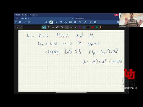
A low-rank Mahalanobis matrix can both learn which directions matter for distance and reduce data to a K-dimensional subspace.

Chapters

0:00 Project Report Deadlines and Peer Feedback Plans

Intermediate project reports are due on Canvas by 10:00 a.m. Tuesday, before class.
Each group should bring printed copies and submit one page per student, including the project goal, progress, figures, and baseline comparisons where relevant.
Tuesday's class includes random projection instruction followed by paired-group report feedback.

7:28 Why Distance Metric Learning Is Needed

A native Euclidean distance may be unreliable when features such as height, weight, and age use different units.
For cities, flight costs can define pairwise distances even when the cities have no useful vector representation.
The goal is to embed objects in a small Euclidean space while preserving meaningful distances for plotting or clustering.

15:15 Similarity Matrices from Graphs, Kernels, and Dot Products

A similarity function assigns large values to similar pairs and small values to dissimilar pairs.
For a graph, similarity can be 1 when two objects share an edge and 0 otherwise.
A Gaussian kernel uses a bandwidth to emphasize nearby points, while a dot product provides a linear similarity.

20:18 Eigenvectors Turn Pairwise Similarities into Embeddings

For N objects, pairwise similarities form an N by N matrix S.
The eigendecomposition S = VΛVᵀ orders orthogonal directions by eigenvalue importance.
Keeping the top K eigenvectors and scaling them by square roots of their eigenvalues gives an N by K embedding.

28:45 Similarity Embeddings and the Dot-Product Interpretation

When S comes from a data matrix A as AAᵀ, the eigenvector construction recovers the best rank-K approximation associated with the SVD.
Graph edges or kernel similarities can be interpreted as encoding alignment in an unknown high-dimensional space.
The same eigenvalue approach can produce an embedding even when the objects have no explicit vector representation.

32:28 Classical MDS Starts from a Pairwise Distance Matrix

Classical multidimensional scaling assumes access to trusted pairwise distances, not to the unknown coordinates that generated them.
The N by N matrix D stores each distance Dᵢⱼ between objects xᵢ and xⱼ.
The desired output is a low-dimensional coordinate matrix Q whose Euclidean distances approximate the entries of D.

37:57 Recovering Inner Products from Squared Distances

Euclidean geometry gives ‖aᵢ − aⱼ‖² = ‖aᵢ‖² + ‖aⱼ‖² − 2aᵢᵀaⱼ.
Rearranging the equation recovers an inner product from squared distances and the squared norms of the two points.
Placing one reference point at the origin lets its distances supply the missing squared norms.

42:40 Centering the Coordinates for Classical MDS

The centering matrix is Cₙ = I − (1/N)11ᵀ, which subtracts the mean from every row of a data matrix.
Centering makes the average embedded point zero, paralleling the centering step used in PCA.
Averaging over possible choices of origin leads to the double-centering construction used by classical MDS.

47:53 Classical MDS: Double-Center, Decompose, and Project

Square each distance elementwise to form D², then compute S = −½ CₙD²Cₙ.
Eigendecompose S and retain the top K eigenvectors and eigenvalues.
Construct coordinates as Q = VₖΛₖ¹ᐟ² to obtain a K-dimensional Euclidean embedding from distances alone.

50:59 What Double-Centering Does to Squared Distances

The −½D² term in the MDS formula comes directly from rearranging the squared-distance identity.
Applying the centering matrix on both sides accounts for the two squared-norm terms while keeping the matrix symmetric.
The resulting coordinates are mean-centered, rather than anchored to a single object at the origin.

55:41 LDA Uses Class Labels to Find Useful Directions

Linear discriminant analysis assumes vector data in Rᴰ and class or cluster labels, but does not trust the raw Euclidean metric.
Its target representation places same-class points close and different-class points far apart.
LDA finds linear projections, so the resulting view reflects separations available through linear transformations.

1:00:43 LDA Measures Between-Class and Within-Class Spread

For each class Sⱼ, compute its mean μⱼ and covariance Σⱼ from deviations x − μⱼ.
Between-class covariance ΣB measures how far class means lie from the overall mean.
Within-class covariance ΣW aggregates class covariances and measures how dispersed the points are inside their classes.

1:06:55 LDA’s Generalized Eigenproblem Separates Classes

LDA seeks directions with large projected between-class variance and small projected within-class variance.
The objective leads to eigenvectors of ΣW⁻¹ΣB, with the top K directions used for projection.
Projecting labeled data onto these directions can reveal class separation in a lower-dimensional view.

1:12:39 Why t-SNE and UMAP Require Careful Validation

t-SNE and UMAP rely on neighborhood similarities and scale parameters, so changing settings can substantially change the displayed structure.
Their low-dimensional layouts can introduce apparent separations, and they do not provide a straightforward map for adding new data points.
Kernel PCA is presented as a more explicit alternative when a nonlinear kernel-based embedding is appropriate.

1:16:29 Validate Embeddings Against Labels and Linear Structure

A visually convincing t-SNE or UMAP plot is not, by itself, evidence that the apparent clusters are reliable.
When class labels are available, LDA provides a linear projection whose separation objective is explicit and can be checked.
The lecture recommends explaining why a nonlinear embedding is appropriate and verifying that its output can be trusted.

1:19:37 Close and Far Pairs Introduce Mahalanobis Metric Learning

Linear metric learning uses labeled close pairs and far pairs, which can be supplied for only part of a dataset.
The goal is to learn a Mahalanobis distance matrix M, generalizing Euclidean distance through affine stretching.
A rank-K M can restrict distance measurement to a K-dimensional subspace; the derivation is deferred to the next lecture.

Transcript excerpt

0:17 Um, so welcome back everyone. So let's get started. Uh, today we're going to talk about uh, distance metric learning. Um, so uh Uh, uh, um, so I'm going to if you look up a survey of the of so distance metric learning, this is probably not the progression we're going to do. We're going to talk about multi-dimensional scaling. Um, uh, uh, um, so linear discriminant analysis and then get to some frameworks for what's called uh, distance metric learning. This is really going to show that if we think of this as an eigen value problem and how to get do learn values

1:05 learn scalings and uh, like um, so low-dimensional approximations using using the eigen value structure, we're going to be able to solve all these problems. So it's a trick you probably have maybe uh, uh, um, so hopefully mostly understand already, but we're going to kind of gradually build it and unlock it for more and more scenarios. So hopefully by the end of the lecture, you feel comfortable saying, I can apply this on here or there and all sorts of stuff. Um before we get started, as usual, let's um, we're going to look at the at the schedule and the big thing is the intermediate report for your project is due on Tuesday. Um, it is due at it's

1:56 due uh, uh, um, so on Canvas at 10:00 a.m. That's before you need to turn in online before class. And in class, you should bring some printed out copies. Okay, bring a a handful of printed out copies per group. Each group should bring a handful. What we're going to do in class on Tuesday is we're going to um Um, so I'm going to give oh, half of a lecture for about half of the period.

This is the start of the transcript. Save this video free for the whole transcript, searchable and time-coded.

Related notes

Summary, takeaways, and chapters were generated by AI from the video's transcript and may contain errors. The video belongs to its creator, UofU Data Science.