UUtah Data Mining | Fall 2026 | L14: Distinct Counting

Overview

The lecture develops approximate distinct counting for data streams, moving from Bloom filters to a hash-minimum estimator and HyperLogLog’s compact leading-zero representation. It then generalizes streaming sketches into mergeable summaries, showing how shared hash functions and compatible data structures support distributed aggregation and time-window queries without losing their space and error guarantees.

Key takeaways

F₀ is the number of stream items with nonzero frequency, and exact computation requires storage linear in M or U, making approximate sketches necessary for large streams.
A Bloom filter guarantees no false negatives but permits false positives; its K-bit array becomes uninformative as insertions saturate the available bit positions.
The minimum of uniform hash values provides a distinct-count signal because repeated items hash consistently, while additional distinct items tend to lower the observed minimum.
The median trick reduces failure probability to roughly δ using O(log(1/δ)) independent estimates, with each estimate using about O(1/ε²) samples.
HyperLogLog compresses a hash minimum by tracking leading zeros, requiring about log log F₀ bits for the relevant counter instead of storing a continuous hash value.
Mergeable sketches enable distributed aggregation and time-window queries: compatible local summaries can be combined without increasing their established space-error trade-off.

Chapters

0:00 Course Updates: Midterm, End-Term Test, and Poster Final

Midterm grades were posted Monday after grading over break; the instructor said the class average was near the intended level.
The end-term test will cover streaming through later-semester material and follow a structure similar to the midterm.
The final assessment is a poster presentation during the scheduled final-period block on the last day.

3:28 Intermediate Project Report and Peer Feedback on November 3

The intermediate report is due the morning before class on November 3 and should document progress, obstacles, and what the group has learned.
The report should be one page per student, so a three-person group submits three pages.
Groups will receive peer feedback in class and schedule roughly seven minutes of instructor feedback the following week.

7:38 Streaming Homework and the Next Dimensionality Reduction Unit

The streaming assignment uses two files of roughly 3 to 4 million lowercase English characters as a proxy for words or IP addresses.
Students will test frequency estimation with sampling, Misra-Gries, and Count-Min Sketch; the assignment is due one week after the lecture.
The next lecture begins dimensionality reduction, reviewing SVD and PCA before moving to more advanced material.

9:50 Streaming Constraints and the Distinct-Count Statistic F₀

A stream presents items A₁ through Aₘ in order, usually in one pass and with memory targeted at O(poly(log M, log U)).
Frequency Fⱼ counts occurrences of item j, while F₀ counts how many items have nonzero frequency.
Exact distinct counting requires space linear in the stream length M or universe size U, motivating relative-error estimates.

16:41 Bloom Filter Setup: One Bit Array and Multiple Hash Functions

A Bloom filter represents a set using a K-bit array initialized to zero, rather than storing each item directly.
It uses T hash functions mapping universe items into the same array, and sets all T indexed bits to one when an item arrives.
The structure is designed for compact set membership, with a controllable false-positive rate.

19:17 Bloom Filter Membership Queries and False Positives

To query q, check the T bits indexed by its hash functions; any zero means q is absent, while all ones returns “present.”
There are no false negatives because insertion never resets a bit, but collisions can produce false positives.
For an item not in the set, a false positive requires all T queried positions to have been set by other items.

26:43 Bloom Filter Saturation Limits for Large Streams

With K bits and an expected set size S, the useful number of hash functions scales approximately with K/S; more detailed tuning minimizes false positives.
As the array fills, queries increasingly return “present”; around K log K random placements with one hash, nearly every bit is occupied.
Bloom filters work well when the expected set is modest relative to allocated bits, but they cannot provide logarithmic-space distinct counting for very large sets.

30:33 Estimating F₀ from the Minimum Uniform Hash Value

Map each distinct stream item through a hash function that behaves like a uniform random value in [0, 1).
Maintain only γ, the minimum hash value seen so far; repeated copies of an item hash identically and do not add new distinct values.
The lecture introduces the estimate F̂₀ = 1/γ − 1, explaining it through the expected spacing of the minimum among distinct uniform samples.

38:24 Averaging Independent Hash Estimates to Reduce Error

Run T independent hash functions and compute a distinct-count estimate for each one.
Average the per-hash estimates to improve accuracy over a single minimum-hash estimate.
The lecture gives a sample requirement proportional to 1/(ε²δ) for relative error ε with success probability at least 1 − δ.

44:40 Median Trick: Lower Failure Probability with Repetition

First configure each estimate for constant success probability, using roughly 1/ε² hash functions per estimate.
Repeat the estimate O(log(1/δ)) times and return the median rather than averaging every run together.
The median remains within the ε-relative-error window unless more than half the independent runs fail, reducing the failure dependence from 1/δ to log(1/δ).

52:25 HyperLogLog’s Leading-Zero Compression Idea

A hash value in [0, 1) can be represented as binary fractional bits, where successive positions contribute 1/2, 1/4, 1/8, and so on.
The smallest hash value is characterized approximately by its leading-zero run, so the sketch can store a zero count instead of a full floating-point value.
That counter uses about log log F₀ bits per estimate, illustrating the compact representation behind the HyperLogLog name.

1:00:20 Distinct Counting Recap: Accuracy Through Sketch Compression

The distinct-count method combines randomized hashing, a minimum statistic, repeated estimates, and median amplification.
The leading-zero encoding replaces continuous values with small integer counters, reducing storage as the distinct count grows.
The lecture presents HyperLogLog as a widely used approach for estimating distinct users, customers, or other large-scale populations.

1:01:32 Mergeable Summaries Preserve Streaming Space and Error

A summary has bounded storage, supports item insertion, and answers approximate queries controlled by parameters such as ε and δ.
A merge operation combines summaries for datasets A and B into a summary for A ∪ B while preserving the same space-error trade-off.
For comparison, Misra-Gries and Count-Min Sketch use space scaling like 1/ε, while the lecture gives sampling and F₀ sketches a 1/ε² dependence.

1:08:23 Distributed Routers and Cloud Machines Merge Local Sketches

Routers can maintain separate summaries of traffic and merge them to estimate activity across multiple devices.
The same approach scales from two routers to hundreds of campus Wi-Fi routers without requiring all raw traffic to be centralized.
Parallel cloud workers can summarize local data first, then combine results while retaining a bounded approximation error.

1:11:38 Recent Time-Window Queries from Hierarchical Summaries

To query a recent interval rather than an entire long-running stream, retain summaries for exponentially growing time blocks such as 1, 2, 4, 8, and 16 units.
The hierarchy uses O(log M) summaries, multiplying the base summary space by only a logarithmic factor.
A time-window query selects disjoint blocks and merges their summaries; boundary handling may introduce limited error.

1:17:13 Merging Samples and Count-Min Sketches with Shared Hashes

For a uniform sample, assign each item a shared random value and retain the K smallest values; merging two samples means selecting the K smallest values from both lists.
HyperLogLog-style minimum summaries can also be merged when the component sketches use the same hash functions.
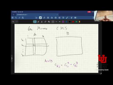
Count-Min Sketch summaries merge by adding corresponding counters, Cᵢⱼ = Cᵢⱼᴬ + Cᵢⱼᴮ; the lecture closes by noting that Misra-Gries also has a merge procedure.

Summary, takeaways, and chapters were generated by AI from the video's transcript and may contain errors. The video belongs to its creator, UofU Data Science.