UUtah CS 6340 NLP | Fall 2026 | Transformers: Self-attention

Overview

The lecture builds the Transformer architecture from token embeddings to self-attention, explaining how query–key dot products produce attention weights and how those weights mix value vectors into contextualized token representations. It then extends the mechanism to multiple heads, explains concatenation and output projection, and connects these operations to encoder–decoder models, decoder-only LLMs, training, and model expressivity.

Key takeaways

Self-attention turns static token embeddings into contextualized representations by scoring every token pair with QKᵀ, applying row-wise softmax, and mixing value vectors with the resulting weights.
The attention score matrix has shape sequence length × sequence length, while multiplying it by V returns one updated representation per input token.
Multi-head attention gives each head separate query, key, and value projections; concatenation followed by WO combines their outputs and restores the model dimension.
Transformer embedding and projection parameters are learned during training; a token such as “bank” can acquire different contextual representations depending on surrounding words.
Attention heads may specialize in different token relationships, but the architecture does not enforce specialization, so redundant heads can emerge and sometimes be pruned.
Scaling query–key dot products by the square root of the key dimension helps keep attention computation numerically stable as that dimension grows.

Chapters

0:00 Practicum Date Change and Transformer Assignment Preview

The second practicum moves to October 19, the Monday after fall break, to allow more time for the practice assignment.
The practicum will focus on Transformers and implementing Transformer-based language modeling; the class will still finish the architecture this week.

2:10 From Token IDs to Learned Static Embeddings

A tokenizer converts input text into an ordered sequence of vocabulary IDs, which retrieve rows from an embedding matrix.
Unlike pretrained Word2Vec vectors, the Transformer’s embedding matrix begins with random values and is learned during training.
The initial embedding for a token is static, so a word such as “bank” has one vector regardless of its sense.

5:00 Contextualizing Tokens for Next-Token Generation

Transformer layers apply nonlinear transformations and use surrounding tokens to produce context-dependent representations.
For “bank,” nearby words such as “river” or “money” can help shape different representations for different senses.
For generation, the final prompt token’s hidden state is projected to vocabulary logits, passed through softmax, and sampled; the new token is appended and the process repeats.

9:30 The 2017 Transformer and Its Cross-Field Impact

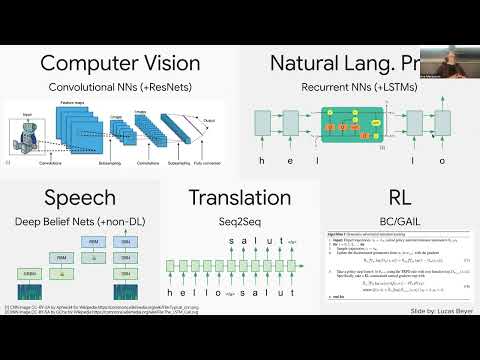
Before Transformers, NLP commonly used RNNs while computer vision commonly used convolutional neural networks.
The 2017 paper “Attention Is All You Need” introduced the Transformer, which became a widely used architecture across machine learning fields.
The lecture notes that modern language models commonly use decoder-only Transformers, despite the original architecture being presented as encoder–decoder.

13:30 Encoder–Decoder Structure and the Encoder Block

The original Transformer uses an encoder to represent a source sequence and a decoder conditioned on that representation to generate output tokens.
An encoder is a stack of encoder blocks; each block combines self-attention with a nonlinear feed-forward transformation.
Self-attention contextualizes every token, while the feed-forward component applies a learned linear projection and nonlinearity.

19:30 Polysemy Motivates Self-Attention

A static embedding cannot distinguish multiple senses of a token, such as the three uses of “basin” shown in the lecture.
Self-attention lets each token representation incorporate information from other tokens in the same input.
For a given token, attention weights indicate how much other input tokens contribute to processing it.

21:00 Creating Query, Key, and Value Projections

For the example sequence “thinking machines,” the input matrix X has one row per token and shape sequence length × embedding dimension.
Learned matrices WQ, WK, and WV project X into query, key, and value representations.
Query and key dimensions must match so their dot products can be computed; the lecture denotes the projected dimension as D2.

26:00 Query–Key Dot Products Form Pairwise Scores

Multiplying Q by K transpose produces a sequence-length × sequence-length score matrix, with one score for each ordered pair of tokens.
In the two-token example, the four scores represent token-to-token comparisons, including each token’s score with itself.
Dot products are treated as learned relevance scores: higher similarity is used as a signal that one token may matter more when processing another.

31:00 Softmax and Scaling Produce Attention Weights

Softmax is applied row-wise to the query–key score matrix, making every attention row sum to one.
The resulting attention matrix contains weights between zero and one and retains the sequence-length × sequence-length shape.
The dot products are scaled by the square root of the key dimension; the lecture presents this factor as an empirical measure for numerical stability.

33:30 Mixing Value Vectors into New Token Representations

Multiplying the attention matrix A by the value matrix V produces a new representation for every input token.
For “thinking,” its output combines value vectors for “thinking” and “machines,” weighted by their respective attention scores.
The output has one row per original token, so attention changes each token’s representation without changing sequence length.

41:30 Self-Attention Parameters, Training, and Matrix Shapes

The input to self-attention can be the initial embedding lookup or the output of the preceding Transformer block.
The embedding matrix and query, key, and value projection weights are learned; in the untrained architecture described, they are initialized randomly.
Attention first computes pairwise token scores with Q and K, then uses those scores to mix projected values into contextualized representations.

47:00 Reading Attention-Matrix Visualizations

An attention matrix can be visualized as a square map over a sentence, with each cell showing a token-to-token weight.
In “He was becoming agitated,” the example shows stronger attention from “he” toward “becoming” and “agitated.”
Such patterns may reflect linguistic relationships, such as a subject attending to its verb, but the model is not explicitly given those labels.

50:00 Multi-Head Self-Attention Learns Multiple Relationships

Each attention head has its own WQ, WK, and WV matrices and independently produces a contextualized representation.
Different heads can learn different patterns, such as subject–verb links, verb–object links, or coreference, without being assigned those roles in advance.
The number of heads is a hyperparameter; the original Transformer used multiple heads, with eight given as an example.

56:00 Concatenating Heads and Projecting to the Model Dimension

Each head produces a sequence-length × head-dimension output matrix, giving multiple representations for every token.
The head outputs are concatenated along their feature columns, producing a sequence-length × (number of heads × head dimension) matrix.
A learned output projection WO maps the concatenated features back to the model dimension so the next block can consume them.

1:01:00 Dimension Choices, Scaling, and Output Projection Questions

Query and key projections need matching dimensions for their dot product, but value vectors may use a different dimension.
The square-root scaling factor is discussed as a stability adjustment whose importance grows with the dot-product dimension.
The output projection both restores the desired model dimension and adds learned flexibility to combine information from attention heads.

1:07:00 Why Heads Can Be Redundant—and What They Learn

No constraint forces separate heads to learn different patterns, so some heads can become redundant; pruning can remove weights while preserving performance.
Large-scale training data and model capacity let Transformers learn many features, including features represented in superposition within dense activations.
The query–key comparison is a learned vector-similarity score rather than statistical correlation, and the attention projections are linear transformations.
Query and key naming follows the matrix orientation needed to produce a square pairwise score matrix over the sequence.

Summary, takeaways, and chapters were generated by AI from the video's transcript and may contain errors. The video belongs to its creator, UofU Data Science.