UUtah Data Mining | Fall 2026 | L15 : SVD + PCA

Overview

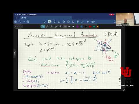
The lecture derives dimensionality reduction through orthogonal projections and the singular value decomposition (SVD), showing how the top k right singular vectors produce the best rank-k approximation under squared reconstruction error. It distinguishes that origin-constrained SVD projection from principal component analysis (PCA): PCA first subtracts the data mean, then applies SVD and projects, allowing the fitted subspace to be offset from the origin.

Key takeaways

Euclidean-distance-based dimensionality reduction assumes feature columns have compatible units, because it combines their squared differences into a single quantity.
The top k right singular vectors of an N-by-D matrix define the best rank-k reconstruction under squared error; the residual squared error equals the sum of squared singular values from k+1 through D.
SVD's projection subspace passes through the origin, so applying it directly to uncentered data can prioritize the data's offset rather than its variation.
PCA addresses the offset problem by subtracting the coordinate-wise mean before SVD, then projecting onto the top k right singular vectors of the centered matrix.
The low-dimensional coordinate mapping returns K values for plotting, while the reconstructed projection returns D values constrained to the selected K-dimensional subspace.

Chapters

0:00 Dimensionality Reduction, SVD, and the Lecture Roadmap

The lecture introduces dimensionality reduction and plans to derive principal component analysis (PCA) through the singular value decomposition (SVD).
SVD is presented as a core linear algebra tool, with later lectures set to cover eigenvalue decompositions and additional reduction methods.
Groups are asked to book instructor feedback meetings for intermediate reports due after November 3.

3:34 High-Dimensional Data as an N-by-D Matrix

The input is a set of n points in R^D, where D may be hundreds, thousands, or millions of dimensions.
Represent the data as an N-by-D matrix A: each of its N rows is a data point, and each of its D columns is a feature.
Reducing D can make later algorithms faster, support visualization in two or three dimensions, and remove dimensions that mainly encode noise.

6:53 Why Feature Units Must Be Compatible

The methods use Euclidean distance, which squares and sums coordinate differences across the D columns.
Features with incompatible units make that sum meaningless; the lecture illustrates the problem with combining population, feet above sea level, and a founding year.
Feature-unit compatibility is treated as essential here, with distance metric learning noted as a later approach for cases where it does not hold.

10:28 Two Outputs: Low-Dimensional Coordinates and Reconstruction

A projection can map a point from R^D to R^K, where K is much smaller than D, such as two or three dimensions for plotting.
The low-dimensional mapping, written as pi-bar, gives K coordinates that are convenient for visualization but cannot be directly compared with the original point.
The reconstruction-style mapping pi returns a point in R^D constrained to lie in a K-dimensional subspace, making reconstruction error measurable.

15:06 Dot Products Define One-Dimensional Orthogonal Projection

For a unit direction u in R^D, the projection of a onto its line is (a · u)u.
The dot product a · u determines the signed distance along the direction, while u sets the projected point's direction.
The unit-length condition on u ensures that it captures direction rather than arbitrary scale, and the result is the closest point on the line.

23:14 Projecting onto a K-Dimensional Orthogonal Basis

A subspace defined by orthogonal unit vectors u1 through uk projects a to the sum of (a · uj)uj across j = 1 to k.
For a two-dimensional subspace, the two projected components are orthogonal, and their sum gives the projection in the original space.
The coordinate mapping pi-bar instead returns the K dot products as a vector, providing coordinates in the chosen basis.

31:48 Choosing the Subspace by Squared Reconstruction Error

The dimensionality-reduction objective selects a K-dimensional subspace F to minimize the sum of squared distances between each data point ai and its projection onto F.
The subspace basis is constrained to consist of orthogonal unit vectors, so the optimization searches over valid K-dimensional projections.
The lecture identifies this least-squares projection objective as the common goal for dimensionality reduction and introduces SVD as its solution.

38:38 SVD Factorizes the N-by-D Data Matrix

SVD writes the input matrix A as U S V-transpose, with U shaped N-by-N, S shaped N-by-D, and V shaped D-by-D.
The diagonal entries of S are singular values, while the remaining entries are zero.
The rectangular shape of S makes portions of U irrelevant to the product when they are multiplied by zero entries.

43:00 Singular Values and Orthogonal Singular Vectors

Singular values are nonnegative and ordered from largest to smallest, so earlier components capture more of the matrix's magnitude.
The columns of U are orthonormal left singular vectors in R^N; the columns of V, equivalently the rows of V-transpose, are orthonormal right singular vectors in R^D.
For reducing the feature dimension D, the right singular vectors have the appropriate dimension and the top k define the projection directions.

47:02 Top-k Right Singular Vectors Give the Best Rank-k Approximation

The SVD can be expanded as a sum of rank-one matrices, each formed from a left singular vector, its singular value, and a right singular vector.
Keeping the first k terms yields A_k, a rank-at-most-k matrix and the best rank-k approximation under the matrix error criteria discussed.
Projecting every row onto the top k right singular vectors produces this low-rank approximation and minimizes the sum of squared projection errors.

53:30 Why Projection Error Is the Sum of the Discarded Singular Values

Expressing each data point in the complete right-singular-vector basis separates its retained first k coordinates from the discarded coordinates.
The retained components cancel when comparing a point with its top-k projection, leaving only terms indexed k+1 through D.
Orthogonality and the Pythagorean theorem reduce total squared reconstruction error to the sum of the squares of the discarded singular values.

1:02:03 Truncated SVD as a Smaller Matrix Product

The rank-k approximation can be formed by retaining only the first k columns of U and V and the corresponding k singular values.
In matrix form, A_k = U_k S_k V_k-transpose; equivalently, it is the sum of the first k rank-one SVD terms.
Setting the remaining singular values to zero explains why the omitted singular-vector components do not contribute to the approximation.

1:06:12 Geometric SVD View: Data Spread Along Principal Axes

The right singular vectors describe orthogonal axes aligned with the data's spread, while singular values indicate the scale along those axes.
In two dimensions, the axes and their scales give an ellipse-like description of the data's variation.
This geometric interpretation assumes the data is centered at the origin, a condition that motivates the distinction between SVD and PCA.

1:09:16 PCA Fits an Offset Subspace Instead of Forcing the Origin

PCA seeks a K-dimensional subspace minimizing squared projection error without requiring that the subspace pass through the origin.
Ordinary SVD on uncentered data restricts its projection directions to subspaces through the origin, which can fit offset data poorly.
The lecture gives positive-valued movie ratings on a 0-to-5 scale as an example where the data may be far from the origin.

1:13:40 PCA Procedure: Center, Run SVD, and Project

Compute the coordinate-wise mean c of the N data points and replace each xi with ai = xi - c.
Run SVD on the centered data matrix A, then project onto the subspace spanned by its top k right singular vectors.
Centering places the mean at the origin; without it, the first singular value can dominate because of the offset rather than meaningful variation.
The lecture previews a follow-up on eigenvalue decompositions and faster approximate or streaming matrix methods for large datasets.

Transcript excerpt

0:17 Um all right so um welcome back let's get started. Um so today we're going to start the section on dimensionality reduction. We're going to we're going to approach this today with the kind of the core uh main principles. We're going to get to principal component analysis through the SVD. Um, okay. So, who feels like they're pretty good with linear algebra? How many people feel like they're they're rusty on linear algebra and and maybe have not taken linear algebra? Uh, okay. Good. Okay. I'm glad it didn't see hands. This is going to this lecture

1:04 is going to review a lot of linear algebra if you've taken foundations of uh of a foundation of day analysis that will cover roughly three lectures from that class today and one lecture. Hopey it's still a good review. Um uh um um so if you've seen this before, if you have not um worked with the the kind of your linear algebra is rusty, this is going to come very fast and so you may want to do some more review outside of class. Um all right. So how many people familiar with the singular value decomposition? Okay. How many people have not used the

1:51 singular value de composition before? Uh okay. Okay. Okay. A few we will we will um review it very very quickly. Um and it will it is kind of the most kind of central tool we'll use in this space and we'll get to the next several lectures. we'll get to kind of more advanced uses of things like the singular value decomposition, the IGEN value decomposition, um, and uses in other ways of doing dimensionality reduction. Um, but I'm going to try to review all of this, get up to PCA today in this lecture from

This is the start of the transcript. Save this video free for the whole transcript, searchable and time-coded.

Related notes

Summary, takeaways, and chapters were generated by AI from the video's transcript and may contain errors. The video belongs to its creator, UofU Data Science.