Stats 401 - Week 5 - Part 1 of 3

Overview

Miles Chen introduces binary classification through logistic regression, showing how the logistic function models class probabilities and how maximum likelihood estimates coefficients. A simulated coronary heart disease example demonstrates odds-ratio interpretation, threshold tradeoffs, confusion matrices, ROC curves and AUC, with R and Python implementations and a cost-based threshold exercise.

Key takeaways

Logistic regression models a binary response with π(x) = 1 / (1 + e^−(β₀ + β₁x)), keeping predicted probabilities between 0 and 1.
The CHD-by-age example estimates an age coefficient near 0.1109, equivalent to about 11.7% higher odds per additional year and about threefold higher odds per decade.
A logistic-regression coefficient changes log-odds, not probability by a fixed amount; the same odds multiplier can produce different probability changes at different starting risks.
Lowering a classification threshold increases positive labels, usually capturing more true cases while also creating more false positives; the appropriate threshold depends on error costs.
ROC AUC evaluates ranking across thresholds, not accuracy at a single threshold; AUC 0.5 represents chance-level ranking, while values below 0.5 can indicate reversed predictions.
R's binomial glm and Python statsmodels' binomial GLM produce matching coefficients for the CHD-age example, and both rely on numerical likelihood optimization.

Chapters

0:00 Classification Goals and Access to the ISL Textbook

Classification predicts a categorical response, assigning new observations to one of several classes.
Miles Chen points students to Introduction to Statistical Learning, noting that UCLA library access provides the full text.
The lesson focuses on logistic regression, a Bayesian classifier, naive Bayes, and k-nearest neighbors.

3:00 Class Labels, Ordinal Variables, and Binary Outcomes

Training data consist of n observations with input vectors x₁ through xₙ and class labels often coded as integers.
Nominal class labels have no numeric order: class 2 is not twice class 1, unlike ordinal categories such as clothing sizes.
The opening logistic-regression example is binary, modeling whether an observation belongs to a category or not.

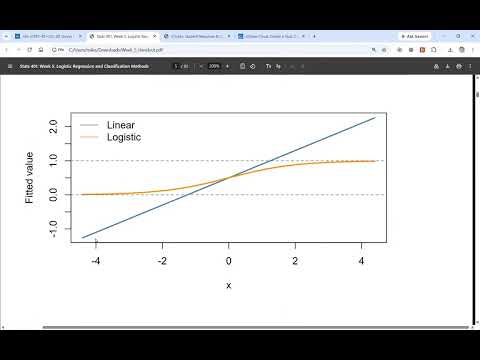
6:30 The Logistic Function Maps Predictors to Probabilities

Linear regression can predict values outside the 0-to-1 range, so it is not suitable for modeling probabilities directly.
The logistic model uses π(x) = 1 / (1 + e^−(β₀ + β₁x)) to constrain predictions between 0 and 1.
The curve approaches 0 for strongly negative linear predictors, 1 for strongly positive ones, and equals 0.5 when β₀ + β₁x = 0.
The logit is the inverse transformation, converting a probability into the linear predictor β₀ + β₁x.

11:30 Bernoulli Responses and the Binomial GLM

For a binary response y, the model treats each observation as a Bernoulli draw with probability π(x) of class 1.
The residual has mean zero and variance π(x)(1 − π(x)), rather than the constant-variance Gaussian error model used in linear regression.
In R, logistic regression can be fit with glm(..., family = binomial); Python's statsmodels provides the corresponding binomial GLM.

14:30 Maximum Likelihood and Numerical Logistic-Regression Fitting

The likelihood multiplies π(x) raised to y by (1 − π(x)) raised to 1 − y across observations.
Taking the log turns the large product into a sum, producing the log-likelihood that software maximizes.
Logistic regression generally has no closed-form coefficient solution, so software uses numerical optimization to find β₀ and β₁.
Perfectly separable data can cause a coefficient, often the slope, to grow without bound.

19:00 Preparing the CHD-by-Age Example with Jitter and Age Bins

A simulated 100-patient dataset relates age to coronary heart disease, abbreviated CHD, with more positive cases at older ages.
Because the response is 0 or 1, many observations overlap in a scatterplot; vertical jitter reveals repeated points.
Age groups such as 20 to 29, 30 to 34, and 60 to 70 summarize the observed CHD proportions, with group midpoints used for plotting.
The grouped proportions rise with age, but the logistic fit is estimated from the original individual 0/1 responses, not from the grouped dots.

25:00 Fitting CHD Logistic Regression in R and Python

The model predicts CHD from age using a binomial GLM in both R and Python's statsmodels formula API.
Both implementations return an intercept near −5.309 and an age coefficient near 0.1109.
The coefficient tests provide strong evidence that the intercept and age effect differ from zero, with reported p-values below 0.0001.
The fitted probability curve captures the increase in CHD risk with age while remaining within the 0-to-1 range.

29:00 Interpreting Age Effects Through Odds Ratios

An age coefficient of about 0.1109 means each additional year increases the modeled log-odds of CHD by about 0.11.
Exponentiating the coefficient gives an odds ratio of about 1.117, or roughly an 11% increase in CHD odds per year.
The lecture reports a 95% coefficient interval around 0.067 to 0.162, which becomes an odds-ratio interval of roughly 1.07 to 1.18.
Confidence intervals can differ slightly by method: the lecture contrasts a Wald interval with a profile-likelihood interval from Python.

36:00 A Ten-Year Age Increase Multiplies CHD Odds by About Three

For a ten-year increase, the odds ratio is exp(10 × 0.1109), approximately 3.03.
The estimated odds rise from about 0.317 at age 37.5 to about 0.960 at age 47.5, illustrating the threefold change.
Observed age-bin proportions show the relationship is not a constant probability increase: odds near 0.33, 0.86, and 3.25 correspond to probabilities near 0.25, 0.46, and 0.77.
Odds can communicate changes in rare outcomes more clearly than small-looking changes in probability, though probabilities remain useful in other ranges.

46:00 The Intercept, Probability Curve, and Classification Thresholds

The intercept describes predicted CHD odds at age zero, which is not meaningful for this dataset because observed ages are about 28 to 69.
Turning probabilities into labels requires a threshold, such as 0.5 or 0.3; lowering it classifies more observations as positive.
Lower thresholds generally increase true positives and false positives while reducing false negatives; higher thresholds tend to do the reverse.
A confusion matrix distinguishes true positives, true negatives, false positives, and false negatives, and the best threshold depends on the consequences of each error.

52:30 ROC Curves and AUC Compare Classifiers Across Thresholds

An ROC curve plots sensitivity, or true-positive rate, against false-positive rate across many classification thresholds.
Sensitivity is TP/(TP + FN); the false-positive rate is FP/(FP + TN), and specificity equals one minus the false-positive rate.
A perfect classifier reaches the top-left corner, while random guessing follows the diagonal and has AUC 0.5.
AUC measures ranking performance rather than classification accuracy or a recommended threshold; an AUC around 0.8 means a CHD case scores higher than a non-CHD case in about 80% of pairs.
An AUC below 0.5 suggests that reversing the model's rankings may perform better than using them as-is.

1:00:40 Multiple Predictors and Choosing a Threshold by Error Cost

Multiple predictors can be added to logistic regression with additional β terms, while multicollinearity remains a possible issue.
In the in-class cost example, a false positive costs 1 unit and a false negative costs 5 units.
The compared threshold choices have calculated costs of 82 and 60 units, favoring the 0.3 threshold in that example.
AUC stays unchanged when the decision threshold changes because it summarizes performance across thresholds rather than the cost of one decision.

Transcript excerpt

0:04 Okay. Uh, I have to click. We got it. All right. Okay. I think I think we're okay. All right. Happy Wednesday. Thanks for uh for joining me here. And today we are going to look at uh classification methods. I have no idea. Not I'm not even able to click that. Okay. Well, that's just the uh the camera is going to be up there. Um Okay. Uh all right. Let's uh let's go ahead and take a look. We're going to um we'll start off with logistic regression. You guys are you are taking what 4041

0:55 right now. Okay. So, you haven't done logistic regression yet? Not yet. Okay. I think that'll be in your next class with I you're gonna have linear regression, which I'm intentionally skipping over. And I think logistic regression may or may not be a part of it. So, um we'll spend a little bit of time on that. And then we'll uh we'll talk about other classification methods. We'll look at the B classifier, naive base classifier, and K nearest neighbors. Okay. All right. Let's go ahead and um and take a look. And again um there uh we're using introduction to statistical learning. There's also this uh textbook. I actually haven't tested the link. I think it still works. It it looks like it.

1:45 Yeah. No, we don't want buy this book. We want we want view and download the full book. Yes. Okay. So, if you are connected via the UCLA network, which should be all of you right now, um it should show UCLA library and um and it should say full access. Okay. So, part of your tuition money goes to pay for our library and all of the kind of digital subscriptions that uh that they get. So, you get access to

This is the start of the transcript. Save this video free for the whole transcript, searchable and time-coded.

Related notes

Summary, takeaways, and chapters were generated by AI from the video's transcript and may contain errors. The video belongs to its creator, Miles Chen.