Stats 102C - Lecture 11 - More Rejection Sampling
 Watch on YouTube →
Overview
Miles Chen explains rejection sampling with non-uniform proposals, deriving the envelope constant and acceptance rule, then applying them to sample a half-normal target using an exponential proposal. The example gives M = sqrt(2e/pi) ≈ 1.315 and an expected acceptance rate of about 76%; Chen also shows how rejection sampling works with an unnormalized kernel and why proposal tail behavior matters.
Key takeaways
- Rejection sampling requires a finite M satisfying f(x) ≤ M g(x) everywhere; the smallest valid M is the supremum of f(x)/g(x).
- For a half-normal target and rate-1 exponential proposal, the density ratio is maximized at x = 1, yielding M = sqrt(2e/pi) ≈ 1.315 and an expected acceptance rate near 76%.
- The probability of accepting any proposal is 1/M, and the density of accepted proposals is exactly the target density f.
- An unnormalized target kernel can be sampled without computing its normalizing constant: bound h(x) by C g(x) and accept with probability h(x)/(C g(x)).
- A proposal with lighter tails than the target may make rejection sampling impossible: the exponential-to-half-normal density ratio diverges in the right tail, so no finite M exists.
- Rejection sampling and importance sampling use related target-to-proposal ratios but serve different goals: rejection produces target draws, while importance sampling weights draws to estimate quantities.
Chapters
- Miles Chen reports a raw midterm median of 78 and a seven-point adjustment, bringing the median to 85.
- The adjusted quartiles are 72 and 92; some recorded scores reach 107.
- Problem 1, part C, which asked students to code Monte Carlo integration, caused the most difficulty.
- Rejection sampling draws candidates from a proposal density g and keeps them with probability f(x)/(M g(x)).
- The envelope condition M g(x) ≥ f(x) must hold everywhere on the target's support.
- A proposal for an unbounded target support cannot be uniform over the whole real line, so a non-uniform proposal is needed.
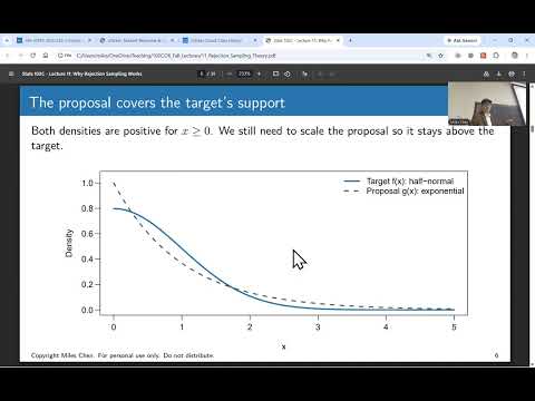
- The target is the half-normal density, defined on x ≥ 0 as sqrt(2/pi) exp(-x²/2).
- The proposal is an exponential distribution with rate 1, whose density is exp(-x) for x ≥ 0.
- Their density ratio is sqrt(2/pi) exp(1/2) exp(-(x-1)²/2), maximized at x = 1.
- The minimum valid envelope constant is M = sqrt(2e/pi) ≈ 1.315, giving an expected acceptance rate of 1/M ≈ 76%.
- Each candidate is drawn from the rate-1 exponential proposal and paired with an independent Uniform(0,1) value.
- Accept x when U < f(x)/(M g(x)); equivalently, accept when U M g(x) < f(x).
- The exponential proposes small positive values more often, while candidates in the far right tail are both uncommon and less likely to be accepted.
- Scaling the proposal density by M creates an envelope that covers the half-normal target at every x.
- A simulation of 100,000 exponential proposals retains 75,849 candidates, close to the theoretical acceptance rate of about 76%.
- The conditional acceptance probability varies with x: values near x = 1 are always accepted, while values near zero are accepted roughly 60% of the time.
- The empirical CDF of accepted draws tracks the half-normal CDF; a Kolmogorov-Smirnov test is suggested as a diagnostic, not a proof.
- Integrating the acceptance probability against g shows the overall acceptance probability is 1/M, and the accepted density simplifies to f(x).
- A target kernel h(x) can be used even when its normalizing constant Z is unknown, provided h is proportional to the target density.
- Choose C so that C g(x) ≥ h(x) everywhere, then accept proposals using h(x)/(C g(x)).
- For the Beta(2,2) kernel h(x) = x(1-x) and a Uniform(0,1) proposal, the maximum of h is 1/4, so C = 1/4.
- The resulting acceptance probability is 4x(1-x), equivalent to the normalized Beta(2,2) density; the overall acceptance rate is Z/C = 2/3.
- Multiplying both h(x) and C by 10 leaves h(x)/(C g(x)) unchanged, so proposal acceptance decisions do not change.
- Changing only the kernel or only the envelope constant can change acceptance probabilities or violate the required bound.
- The iClicker exercise reinforces that rejection sampling depends on the ratio of the target kernel to its scaled proposal.
- Reversing the earlier example uses an exponential target and a half-normal proposal.
- The exponential tail decays more slowly than the half-normal tail, so f(x)/g(x) grows without bound as x approaches infinity.
- No finite envelope constant M can make M g(x) cover the exponential target over its entire right tail.
- A proposal must have tails at least as heavy as the target wherever the target has positive density.
- A useful proposal is easy to sample from, supports the entire target, yields a finite M, and keeps M small to avoid excessive rejection.
- For routine work, use a computer's built-in generator when one directly samples the desired distribution.
- Rejection sampling generates target-distributed draws and discards proposals; importance sampling retains proposals and weights them to estimate expectations or integrals.
- Importance-sampling weights f/g may exceed 1, while the rejection acceptance ratio f/(M g) is bounded between 0 and 1.
Transcript excerpt
0:02 I hope Wait, sorry, let me Okay, all right. So we will continue on looking at rejection sampling. I just posted scores from the midterm exam and uh I did uh I uh the raw median was a 78, so I added seven points to everybody's score. So that brings the median up to 85. I think um Q3 is 92 and Q1 is 72. Um So yeah, 72, 85, 92.
0:50 Um and then, you know, some students got 107. Um so the score that you see in the uh in the grade book already includes that seven point um uh adjustment. And um and that's that. Hey, I don't have office hours today, but um you can come see your exams at any of my in-person office hours uh and things like that. So um So that's that. Um Yeah, overall, I think the one that uh the problem that gave students the most difficulty was the uh part C of problem one where you had to write the code to
1:39 um do the Monte Carlo um uh the code to do the Monte Carlo integration. So uh so maybe I'll have to uh cover that that one aspect uh a bit again. But um but most the other ones overall pretty good, I think. Okay. So, um so we've been talking about rejection sampling, and again, this is all uh because we want to be able to generate a sample from the target distribution, okay? And so, in Wednesday's lecture, um what we showed was you can have a target distribution,
2:26 and uh instead of directly drawing samples from that target distribution, um you draw values from a different distribution. Like uh and on Wednesdays, we were drawing from a uniform distribution. And what we did was we
This is the start of the transcript. Save this video free for the whole transcript, searchable and time-coded.
Related notes
Summary, takeaways, and chapters were generated by AI from the video's transcript and may contain errors. The video belongs to its creator, Miles Chen.