Stats 102C - Lecture 13 - Introducing Markov Chains
 Watch on YouTube →
Overview
Miles Chen introduces Markov chains as a way to generate dependent samples when methods such as rejection sampling struggle, illustrated by a folded Student t distribution with 3 degrees of freedom and an exponential proposal whose tail is too light. He defines transition matrices and the Markov property, demonstrates weather, Ehrenfest urn, and random-walk chains, then uses matrix multiplication to show that the weather chain converges to a stationary distribution of 0.75 sunny and 0.25 not sunny.
Key takeaways
- A folded Student t distribution with 3 degrees of freedom has heavier tails than an exponential proposal, so exponential-based rejection sampling cannot satisfy a finite envelope bound across the whole domain.
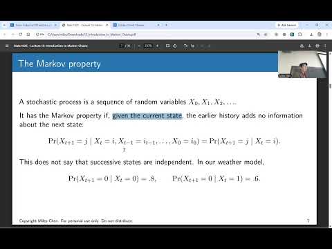
- The Markov property makes the current state sufficient for determining the next-state distribution, even though successive states in the chain are dependent.
- For the two-state weather matrix [[0.8, 0.2], [0.6, 0.4]], starting sunny gives a probability of 0.76 of being sunny after two transitions.
- A Markov chain simulation must choose its transition probabilities based on the current state; repeatedly sampling from [0.8, 0.2] instead produces independent draws, not the weather chain.
- In the Ehrenfest urn with N balls, the count in urn A moves from i to i - 1 with probability i/N and to i + 1 with probability (N - i)/N.
- The weather chain converges to a stationary distribution of [0.75, 0.25], regardless of whether it begins sunny or not sunny.
Chapters
- Miles Chen motivates Markov chain Monte Carlo as a tool for sampling from complicated, especially multivariate, distributions.
- For a folded Student t distribution with 3 degrees of freedom, an exponential proposal decays faster in the tail than the target, so no finite scaling factor M can keep the proposal above the target everywhere.
- Rejection sampling then underproduces tail values; an alternative sampling strategy is needed for distributions without a practical inverse CDF or rejection sampler.
- A Markov chain generates a sequence in which each next state depends on the current state, unlike the independent draws used in earlier sampling methods.
- The Markov property says the distribution of X at time t + 1, given the full history, depends only on X at time t.
- In the weather example, sunny today gives an 0.8 probability of sunny tomorrow, while not sunny today gives a 0.6 probability.
- A state space is the set of values a chain can take; examples include {0, 1}, the integers, or the real numbers.
- A time-homogeneous chain uses the same transition probabilities at every time step; climate change is an example of why a model might instead vary its probabilities over time.
- The weather transition matrix has rows [0.8, 0.2] and [0.6, 0.4], with each row summing to 1 and representing next-state probabilities conditional on the current state.
- At each step, select the transition-probability row for the current state, draw a random value, and use that row to determine the next state.
- Using the [0.8, 0.2] row regardless of the current state creates independent draws and does not simulate the specified Markov chain.
- A 10,000-step simulation recovers transition frequencies near 0.8 and 0.2 from state 0, and near 0.6 and 0.4 from state 1.
- The Ehrenfest model tracks the number of balls in urn A, with states 0 through N, as one randomly selected ball moves between two urns at each step.
- With N = 4 and 2 balls in urn A, the next state is 1 or 3, each with probability 0.5.
- From state i, the chain moves to i - 1 with probability i/N and to i + 1 with probability (N - i)/N; at state 4 it must move to 3, and at state 0 it must move to 1.
- A random walk adds +1 with probability p and -1 with probability 1 - p at each step, so the next position depends only on the current position.
- From position 5, the chain moves to 6 with probability p or to 4 with probability 1 - p.
- In a simulated 1,000-step fair walk, the endpoint can differ from zero despite equal probabilities of winning and losing at each step.
- The vector Q_t records the probability of occupying each state at time t, distinct from a transition matrix row, which gives probabilities conditional on a current state.
- For the weather chain, starting at state 0 means Q_0 = [1, 0], and after one transition Q_1 = [0.8, 0.2].
- The distribution at a later time can be calculated by combining all possible paths, rather than predicting a single realized state.
- Starting sunny, the probability of sunny at time 2 is 0.8 × 0.8 + 0.2 × 0.6 = 0.76; the probability of not sunny is 0.24.
- Thus Q_2 = [0.76, 0.24], equivalent to summing the probabilities of the paths 0 to 0 to 0 and 0 to 1 to 0.
- Repeated matrix multiplication updates the state-probability vector efficiently without drawing random samples or enumerating an increasingly large path tree.
- For the weather matrix with transitions 0.8/0.2 from sunny and 0.6/0.4 from not sunny, repeated updates approach [0.75, 0.25].
- The limiting distribution is the same whether the chain starts in state 0 or state 1, illustrating the stationary-distribution idea previewed for the next lecture.
- The Friday lecture will be prerecorded, with no in-person class or iClicker quiz; Miles Chen says slides and the recording will be posted.
Transcript excerpt
0:02 All right. Well, uh good morning and happy Wednesday of week five. Um So, uh Friday, day before Halloween, uh I will not come to campus. I will post a pre-recorded video for the lecture. So, just uh please be sure to watch that. Uh no in-person class, no iClicker quiz. That's that, okay? But, uh but I'll post the uh I'll post the video and the lecture slides and stuff. Okay. All right. Today, uh we are going to introduce Markov chains, okay?
0:52 So, on Monday, we sampled from some bivariate distributions. And uh and you know, we eventually our goal is going to be to uh draw samples from multivariate distributions cuz we have, you know, these complicated problems and we want to get a sample from them. And uh a common way, just cuz they get real complicated, one way is to do Markov chain Monte Carlo. And so, before we can get into that, we got to learn what a Markov chain is. And so, we'll talk about all of that stuff and then we'll run a simulation of that and things like that. Okay. So, this is just like a
1:39 a an example of how uh you know, like this isn't even a multivariate example. This is just a unit univariate uh example where you can have this um distribution. So, if you wanted to do a T distribution with 3 degrees of freedom, uh this is what the PDF looks like, okay? This is something very kind of unfamiliar to us. But, uh but yeah, it it looks like this. There's not even an E in the uh the T distribution with 3 degrees of freedom. Um and you can say, "All right, well, uh what if we want to do rejection sampling?" And we say, "All right, let's
This is the start of the transcript. Save this video free for the whole transcript, searchable and time-coded.
Related notes
Summary, takeaways, and chapters were generated by AI from the video's transcript and may contain errors. The video belongs to its creator, Miles Chen.