Stats 102C - Lecture 12 - Basic Multivariate Sampling
 Watch on YouTube →
Overview
Miles Chen develops basic multivariate sampling by showing how to sample dependent discrete pairs, generate independent standard normals with the Box-Muller transform, and convert those normals into a correlated bivariate normal. The lecture also demonstrates how shuffling one column preserves marginal frequencies but destroys the original joint dependence, and derives the covariance of linear combinations of independent normals.
Key takeaways
- A discrete joint PMF can be sampled by flattening its cells in a fixed order and assigning each cell an interval whose length equals its probability.
- Shuffling one column of paired observations preserves both marginal distributions but changes the joint distribution by breaking the original dependence.
- The Box-Muller transform generates independent standard normals using two independent uniforms: theta = 2pi U1, R = sqrt(-2 log(1 - U2)), then Z1 = R cos(theta) and Z2 = R sin(theta).
- A bivariate normal with correlation rho can be built from independent standard normals using X = muX + sigmaX Z1 and Y = muY + sigmaY(rho Z1 + sqrt(1 - rho²) Z2).
- For X = Z1 + Z2 and Y = Z1 - Z2 with independent standard normals, both variables have variance 2 and covariance 0; joint normality makes them independent, but they are not standard normal.
Chapters
- Miles Chen connects earlier Monte Carlo estimation and univariate sampling methods, including inverse CDF and rejection sampling, to the goal of generating multivariate draws.
- A multivariate draw contains multiple values, such as X and Y, whose dependence must be preserved when their covariance is nonzero.
- The lecture moves from discrete joint probability mass functions to Box-Muller normal sampling and correlated bivariate normal generation.
- For binary X and Y, the joint probabilities are 0.2, 0.6, 0.1, and 0.1, with outcomes ordered as 00, 10, 01, and 11.
- Flatten the joint table in an arbitrary fixed order, then divide the interval from 0 to 1 into segments matching the cell probabilities.
- A uniform draw of 0.25 selects outcome 10, while a draw of 0.7 selects outcome 01.
- Joint sampling matters because multiplying marginal probabilities would give the wrong cell probabilities when X and Y are dependent.
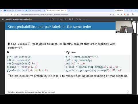
- Flatten a multivariate probability grid, compute its cumulative sum, and align each probability interval with the corresponding X and Y values.
- In R, use findInterval; in Python, use searchsorted to locate a uniform draw in the cumulative probabilities.
- Set the last cumulative probability explicitly to 1 to avoid floating-point rounding problems that could leave the final interval uncovered.
- A 10,000-draw simulation produces empirical joint frequencies close to the target table, though random sampling does not reproduce the exact probabilities.
- Shuffling the Y column after generating 10,000 paired observations leaves the X and Y column totals unchanged.
- The shuffle breaks the original row-by-row pairings, so the joint frequencies change and X and Y become approximately independent.
- The example distinguishes marginal frequencies, which describe each column separately, from joint frequencies, which describe paired outcomes.
- For independent standard normals Z1 and Z2, their joint density contains the term exp(-(Z1² + Z2²)/2), which has circular symmetry.
- Switch to polar coordinates with Z1 = R cos(theta) and Z2 = R sin(theta); the absolute Jacobian determinant contributes a factor of R.
- The resulting density factors into an exponential distribution for S = R², with rate 1/2, and a uniform distribution for theta on [0, 2pi).
- Because the transformed density factors, S and theta can be sampled independently before converting back to Z1 and Z2.
- Generate independent uniforms U1 and U2, set theta = 2pi U1 and S = -2 log(1 - U2), then take R = sqrt(S).
- Compute Z1 = R cos(theta) and Z2 = R sin(theta) to obtain a pair of independent standard normal values.
- For numerical accuracy in code, Chen recommends using log1p for the logarithm involving 1 minus a uniform draw.
- A simulation of 1,500 pairs gives sample means near 0, variances near 1, and correlation near 0; the polar-coordinate picture explains the radial and angular roles of the uniforms.
- To obtain a normal variable with mean mu and variance sigma squared, transform a standard normal Z as mu + sigma Z.
- Independent rescaling alone cannot create covariance, so the bivariate construction shares Z1 between X and Y.
- Use X = muX + sigmaX Z1 and Y = muY + sigmaY(rho Z1 + sqrt(1 - rho²) Z2), where Z1 and Z2 are independent standard normals.
- The construction gives covariance rho sigmaX sigmaY and preserves the requested marginal variances; rho = 0 yields independent components, while rho approaching 1 makes Y rely increasingly on Z1.
- Chen applies the transform to Box-Muller values using means muX = 1 and muY = 2, unit standard deviations, and correlation rho = 0.7.
- The X coordinate is formed from Z1, while Y combines rho times Z1 with sqrt(1 - rho²) times Z2.
- The resulting scatter has the intended positive association and demonstrates how independent normal draws can be converted into a joint distribution with a specified covariance.
- For independent standard normals Z1 and Z2, the class considers X = Z1 + Z2 and Y = Z1 - Z2.
- Each variable has mean 0 and variance 2, since the variances of the two independent terms add.
- Their covariance is Var(Z1) - Var(Z2) = 0, because the cross-covariances vanish and both standard normals have variance 1.
- Since X and Y are jointly normal, zero covariance implies independence; each has distribution N(0, 2), not standard normal.
Transcript excerpt
0:02 All right. Happy Monday, 8:00 a.m. Thanks for for being here and enjoying me for lecture 12, multivariate sampling. Okay, so um so far we've kind of the story of the course so far is um we started off with some Bayesian ideas and the the reason why I started off with Bayesian ideas is because I wanted to show that um doing posterior inference uh is is hard and um and it often requires doing an integral or you can take the money Carlo approach and by um generating a random sample
0:53 uh you can estimate, you know, quantities. And so we did a little bit of money Carlo estimation and things like that where we used random samples to um to estimate those quantities. And then we talked about, well, how do we get those random samples? And uh and the short of it is a lot of this stuff is already built into your computer with the random number generator. But we talked a little bit about how some of these random number generators work. And we did inverse CDF and rejection sampling and things like that. And those were all ways for us to get univariate random samples. And uh and today now we want to say we want to draw um multivariate samples where one draw will consist of
1:42 more than one value, okay? And uh and when we do that, we don't necessarily want X and Y to be independent, okay? If If X and Y are independent, it would be simple. We just generate X and And independently we generate Y and then we would have no problem. But a lot of times we want to show that there's some kind of covariance between them. And so um this it gets uh we're going to start off with
This is the start of the transcript. Save this video free for the whole transcript, searchable and time-coded.
Related notes
Summary, takeaways, and chapters were generated by AI from the video's transcript and may contain errors. The video belongs to its creator, Miles Chen.