Stats 102C - Lecture 19 - Multivariate MCMC concepts
Overview
Miles Chen extends Metropolis sampling from scalar values to vectors, using a bivariate normal target with correlation 0.8 to show how joint proposals can be rejected frequently and become inefficient in higher dimensions. He introduces Gibbs sampling as an alternative: update one coordinate at a time from its conditional distribution, which for this bivariate normal has variance 1 − 0.8² = 0.36 and requires no rejection step.
Key takeaways
- For a symmetric Metropolis proposal, the acceptance probability is min(1, target density at the proposed vector divided by target density at the current vector); log densities make the calculation numerically convenient.
- A proposal that is too narrow can produce high acceptance but poor exploration, while a proposal that is too broad can trigger frequent rejections.
- Joint proposals become harder to accept as the number of coordinates grows, especially when a proposal must move all coordinates to a collectively plausible location.
- Gibbs sampling replaces joint proposals with coordinate-wise draws from conditional distributions, using updated values as the chain proceeds through each sweep.
- For a standardized bivariate normal with correlation 0.8, each coordinate conditional on the other has variance 0.36 and a mean equal to 0.8 times the fixed coordinate.
- Gibbs sampling requires no rejection when each coordinate is sampled exactly from its conditional distribution, but deriving those conditionals can be the hardest part of applying the method.
Chapters
- Metropolis-Hastings can target a distribution using values proportional to its density, so a difficult normalizing constant is not required.
- A Markov chain should converge to the target as its stationary distribution, but poor proposal scale can make practical convergence very slow.
- In multivariate sampling, each state is a vector, and a joint proposal changes multiple coordinates at once.
- The example target is a two-dimensional normal centered at (0, 0), with variance 1 in each coordinate and correlation 0.8.
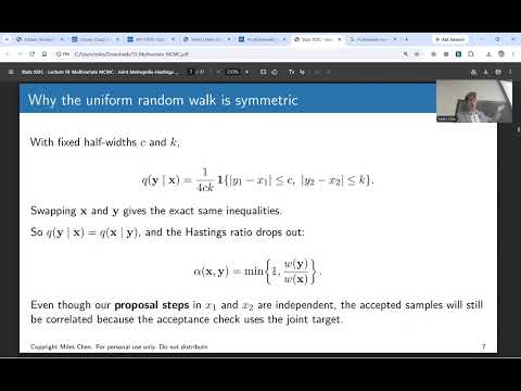
- A uniform proposal selects a point in a rectangle centered on the current state, with half-widths c and k for the two coordinates.
- A multivariate normal proposal can also be centered at the current state; symmetric proposals cancel in the Metropolis-Hastings ratio.
- Moving from (1, 1) to (1.6, 0.4) changes the log target density from about −0.55 to −2.35.
- The log-density difference is −1.8, giving an acceptance probability of exp(−1.8) ≈ 0.1653.
- Compare log(U) with the log acceptance ratio to avoid calculating extremely small density values directly.
- In the uniform-proposal animation, 10 of 40 proposals are accepted, with repeated rejections leaving the chain at its current state.
- The normal-proposal run accepts 21 of 40 proposals, illustrating that the proposal distribution affects both acceptance and movement.
- Tiny steps can be accepted often but explore little; oversized steps explore farther but are frequently rejected.
- When all coordinates are proposed together, the full vector is rejected if its proposed location has a poor joint target density.
- As an intuition rather than a general acceptance formula, independent 10% chances of a good proposal for each coordinate yield about 1% for two coordinates and 0.1% for three.
- A proposal covariance aligned with the target can help, but the target covariance is often unknown and becomes harder to estimate in many dimensions.
- Gibbs sampling holds all other coordinates fixed and samples the selected coordinate from its conditional distribution.
- For two variables, the chain alternates between sampling X1 given X2 and X2 given the newly updated X1.
- A full sweep updates each coordinate once, using the most recently available values for the other coordinates.
- For standardized bivariate normal variables with correlation ρ, X1 given X2 is normal with mean ρX2 and variance 1 − ρ².
- With ρ = 0.8, each conditional variance is 0.36; the corresponding conditional standard deviation is 0.6.
- The animation shows alternating horizontal and vertical draws as each coordinate is sampled from its changing conditional normal distribution.
- Exact conditional draws are accepted automatically, avoiding the repeated accept-or-reject decisions of joint Metropolis proposals.
- The central challenge is deriving and sampling from each conditional density; this is straightforward for the bivariate normal but can be difficult for complex joint models.
- Hierarchical Bayesian models are a useful application because their structure often makes the conditional distributions available.
- Treating the conditional distribution as a proposal leads to an acceptance probability of 1 when the draw is generated from the correct conditional.
- Gibbs sampling trades joint vector proposals for sequential coordinate updates, with each sweep updating coordinates in turn.
- The lecture closes by previewing hierarchical models as the next topic and a setting where Gibbs sampling can be especially effective.
Transcript excerpt
0:00 record. All right. Uh, good morning and happy Monday. I feel like I'm barely I had a rough morning this morning. Uh, but anyway, uh, I'm here and you guys are here and we're still learning MCMC and this is great. Okay. So, um we So, okay. Well, actually, I guess two weeks ago, last week you guys took the midterm and then it was also a holiday and then we just did like this deciphering thing which was kind of fun maybe. Um but then yeah I guess two weeks ago then we had the Metropolis uh algorithm metropolis Hastings and we
0:48 showed like oh okay um even if you don't know the full PDF if you have something proportional to it okay which is often very helpful in um the basian case uh or just like whenever the denominator is really hard to figure out that's okay you can use the metropolis algorithm and you can start at an arbitrary point. Doesn't even have to be good. And eventually it'll get to the right areas and then you can let it run and you'll get a sample. Okay. And we saw a few things like um so the properties of that metropolis markoff chain says that in the long run it's going to the sample you draw will look like the actual sample or actual
1:38 distribution will reflect that that's what it's uh the stationary distribution is equal to the target distribution. So theoretically that's what we should get. But at a practical level, if your proposal distribution isn't good in that like you're proposing too far away or you're proposing too close and you don't get the width quite right, um it takes a long time, uh it could take a really long time to get a a sample that works. Okay, that
This is the start of the transcript. Save this video free for the whole transcript, searchable and time-coded.
Related notes
Summary, takeaways, and chapters were generated by AI from the video's transcript and may contain errors. The video belongs to its creator, Miles Chen.