STAT 638 (Fall 2026), Lecture 28
 Watch on YouTube →
Overview
Samiran Sinha closes a quiz review on spike-and-slab variable selection, then develops Bayesian inference for multivariate normal data with vector mean and covariance matrix. He derives the conditional posterior for the mean, introduces the Wishart and inverse-Wishart distributions as matrix analogues of chi-square and inverse-gamma distributions, and demonstrates Wishart simulation.
Key takeaways
- A spike-and-slab prior expected model size of 5 is a prior expectation, not a constraint: with 50 candidate predictors, the posterior average model size can be about 12 if supported by the data.
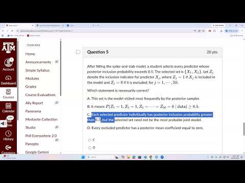
- Predictors with individual posterior inclusion probabilities above 0.5 need not form the single most probable joint model, because marginal inclusion probabilities do not determine joint model probabilities.
- With a multivariate normal likelihood and normal prior for the mean, the conditional posterior precision is the sum of prior precision and N times data precision.
- The precision matrix encodes partial association among features and is useful for building conditional-dependence graphs in high-dimensional settings.
- The Wishart distribution generalizes the chi-square distribution from scalar sums of squares to positive-definite random matrices; when P=1, it reduces to a scaled chi-square distribution.
- The inverse-Wishart distribution serves as a conjugate prior for a multivariate normal covariance matrix, and inverse Wishart draws can be generated by inverting Wishart draws.
Chapters
- With 50 candidate predictors, a prior expected model size of 5 does not force the posterior average number of nonzero coefficients to equal 5.
- A posterior sample average of about 12 included predictors can be supported by the data, even when the prior expectation is 5.
- Increasing the number of MCMC iterations improves sampling accuracy but does not push the posterior model size toward the prior expectation.
- The event that X1 and X2 are included and X3 through X50 are excluded is a joint probability involving all 50 inclusion indicators.
- The probability that X1 and X2 are included alone does not impose any condition on the remaining predictors.
- Selecting predictors with posterior inclusion probabilities above 0.5 does not guarantee that their combined model is the most frequently visited posterior model.
- Sinha reviews block sampling and collapsed Gibbs sampling alongside Metropolis-Hastings.
- A random-walk proposal's standard deviation affects both autocorrelation among sampled values and convergence behavior.
- The quiz review concludes the Chapter 10 material on MCMC computation.
- Chapter 7 shifts from one scalar outcome to a P-component outcome vector modeled as multivariate normal with mean vector μ and covariance matrix Σ.
- The multivariate normal density replaces the scalar squared deviation with a quadratic form involving Σ inverse, and uses the determinant of Σ in its normalizing constant.
- For N independent observations, each Yi is a P-dimensional vector and the joint likelihood combines N multivariate normal densities.
- Sinha assigns the unknown mean vector θ a multivariate normal prior with known mean μ0 and covariance matrix Λ0.
- Combining the prior quadratic form with the data likelihood yields a conditional normal posterior for θ given Σ and the observations.
- The posterior covariance is (Λ0 inverse + NΣ inverse) inverse, and the posterior mean weights μ0 and the sample mean using their respective precision matrices.
- Precision is the inverse of a covariance matrix, and posterior precision combines prior precision with N times the data precision.
- For high-dimensional features, the precision matrix relates to partial correlations, which measure association after accounting for other variables.
- Precision matrices support conditional-dependence graphs and applications such as genomic analysis and control theory.
- For independent scalar normal observations, sums of squared standardized values follow a chi-square distribution; centering by the sample mean reduces the degrees of freedom from N to N−1.
- For P-dimensional standard normal vectors, summing outer products YiYi transpose produces a Wishart random matrix.
- The Wishart distribution generalizes chi-square to positive-definite matrices, with a density involving a determinant and a trace; the scalar case P=1 recovers a scaled chi-square distribution.
- If independent Wishart matrices share scale matrix Ω, their sum is Wishart with degrees of freedom equal to the sum of the individual degrees of freedom.
- A full-rank linear transformation of a Wishart matrix produces another Wishart matrix with a transformed scale matrix.
- Partitioning a Wishart matrix yields Wishart-distributed diagonal blocks, a Wishart Schur complement with adjusted degrees of freedom, and a matrix-normal conditional distribution for an off-diagonal block.
- A gamma random variable can be reparameterized as a scaled chi-square variable, making inverse-gamma analogous to inverse chi-square.
- The inverse-Wishart distribution extends the inverse-gamma role to covariance matrices and provides a conjugate prior for Σ in multivariate normal models.
- Taking the matrix inverse of a Wishart-distributed positive-definite random matrix gives an inverse-Wishart distribution.
- Sinha checks that the specified scale matrix is positive definite by verifying that all its eigenvalues are positive.
- R's rWishart function generates random matrices from a Wishart distribution using a selected degrees-of-freedom value and scale matrix.
- Repeated draws can be averaged elementwise to examine their empirical mean and variance; inverting each draw produces inverse-Wishart samples.
Transcript excerpt
0:01 Sinha, Samiran: Today, I will discuss the remaining questions of quiz number 4, and then we'll talk about some parts of Chapter 10. Sinha, Samiran: Chapter 10, MCMC Completation. Sinha, Samiran: All right, so question 3 says, a student fits the following model to Y… With 50 candidate predictors.
1:03 Sinha, Samiran: After discarding, Barney, the student finds that the average number of non-zero coefficients. Sinha, Samiran: Across posterior draws is approximately Approximately 12. Sinha, Samiran: Average number of non-zero coefficients across posterior draws is approximately 12. Sinha, Samiran: A is not the correct answer. B, the argument specifies a prior expectation. Sinha, Samiran: The data can support a postage average model size of 12, Sinha, Samiran: There is no specification of the argument. Sinha, Samiran: Every posterior draw must contain exactly 5 non-zero coefficients.
2:01 Sinha, Samiran: coefficient, so the student counted incorrectly, so this is not the correct answer. C is not the correct answer. A is not the correct answer. Increasing NITAR sufficiently will force the posterior average model size towards 5. That is also not the correct answer. Now, B, let me see what was B. Sinha, Samiran: Okay, so AACD are 3 wrong things. Sinha, Samiran: Look, YD is incorrect. Increasing NT here, number of iterations, sufficiently will force the posterior average model size towards 5. That is also not true, okay? So, we… we do not enforce that Sinha, Samiran: expected, size will be 5. This is the prior information. So the argument specifies the prior expectation. The data can support a posterior average model size of 12. So, this is fine. This is correct answer, B. Sinha, Samiran: Although this is our prior expectation, your posterior expected value could be different from the prior value.
3:09 Sinha, Samiran: Question for a student fills the following model.
This is the start of the transcript. Save this video free for the whole transcript, searchable and time-coded.
Related notes
Summary, takeaways, and chapters were generated by AI from the video's transcript and may contain errors. The video belongs to its creator, Samiran Sinha.