STAT 638 (Fall 2026), Lecture 23

Overview

Samiran Sinha distinguishes frequentist standard error—which describes estimator variability across hypothetical repeated samples—from Bayesian posterior standard deviation, which describes parameter uncertainty conditional on the observed data. He then develops Bayesian variable selection for linear regression using G-prior marginal likelihoods, demonstrates posterior model and inclusion probabilities on a three-predictor example, and motivates Gibbs sampling and model averaging when exhaustive model enumeration becomes impractical.

Key takeaways

Frequentist standard error estimates the repeated-sampling standard deviation of an estimator, whereas Bayesian posterior standard deviation measures uncertainty about a parameter conditional on the observed data.
For Bayesian regression model selection, posterior model probability is proportional to the model’s marginal likelihood multiplied by its prior probability; equal model priors make posterior rankings depend on marginal likelihood.
In Sinha’s three-predictor simulation, the model containing only X₂ receives the strongest support across G = 5, N, and 40, partly because X₂ is strongly predictive and correlated with X₁ and X₃.
Posterior inclusion probability for a predictor is the sum of probabilities of all models containing it; it is not part of a set of probabilities that must sum to one across predictors.
Exhaustive selection over 20 predictors requires considering 1,048,576 models, motivating Gibbs sampling to explore model space without calculating every model’s probability.
Bayesian model averaging combines predictions by weighting each candidate model’s predictions by its posterior probability, rather than relying only on the single highest-probability model.

Chapters

0:00 Linear Regression Review and the G-Prior Coding Assignment

Sinha opens Chapter 9 by revisiting linear regression and compares classical and frequentist estimates with Bayesian results from the previous lecture.
He asks students to check or correct code using a G prior because its computed results appeared inconsistent with package output.

2:00 Frequentist Standard Error Across Repeated Samples

For the model Y = μ + ε, the classical estimator is the sample mean, with variance σ²/N and standard error estimated by σ̂/√N.
The standard error estimates the standard deviation of μ̂ across many hypothetical samples of size N drawn from the same population.

8:00 Bayesian Posterior Standard Deviation for the Mean

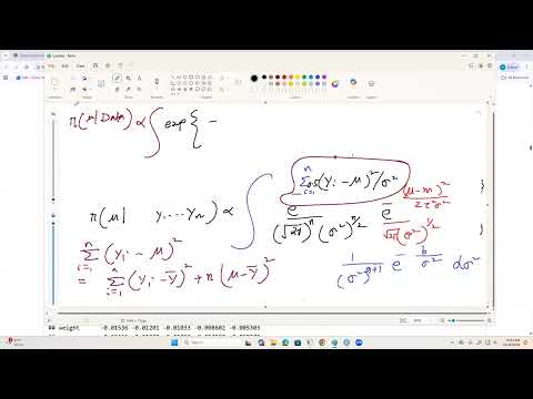
Sinha sets up normal observations with unknown mean μ and variance σ², a normal prior for μ, and an inverse-gamma prior for σ².
Integrating out σ² yields a marginal posterior for μ; completing the square in the likelihood and prior reveals its location-scale form.
The derivation tracks powers of σ² from the likelihood, the prior on μ, and the inverse-gamma prior before applying the gamma integral.

23:00 Scaled-t Posterior and the Meaning of Bayesian Uncertainty

The marginal posterior for μ can be expressed as a scaled Student t distribution, with degrees of freedom tied to N and the inverse-gamma prior parameter.
A Bayesian posterior standard deviation describes uncertainty in the parameter conditional on the observed data; a frequentist standard error describes variability over repeated samples.
The two quantities can be numerically close, as in the earlier example, but neither is necessarily larger and changing the Bayesian prior can change posterior spread.

27:58 Bayesian Model Selection with Predictor Inclusion Indicators

Bayesian model selection chooses models using posterior probabilities proportional to marginal likelihood times prior model probability.
For each of P predictors, an indicator Zⱼ is 1 when the predictor is included and 0 when excluded; P predictors define 2ᴾ possible models.
A vector such as Z = 1010 selects predictors X₁ and X₃ and uses the corresponding two columns of the design matrix.

31:00 G-Prior Marginal Likelihoods in a Three-Predictor Example

Sinha calculates marginal likelihoods for linear regression using a G prior on regression coefficients and an inverse-gamma prior on σ².
With three predictors there are eight indicator combinations; excluding the intercept-only null model leaves seven candidate models in the example.
Assuming equal prior probabilities for models, the model containing only X₂ has the largest posterior probability, consistently across G = 5, G = N, and G = 40.
Although the simulated truth includes X₁ and X₃ with weaker effects, X₂ is strongly predictive and correlated with the other predictors, while marginal likelihood also favors parsimonious models.

40:09 Posterior Inclusion Probabilities for Individual Predictors

A predictor’s posterior inclusion probability is found by summing the posterior probabilities of every model that contains it.
For G = N, the example gives X₁ an inclusion probability of about 0.195 and X₂ about 0.973, making the evidence for X₂ much stronger.
Inclusion probabilities for X₁, X₂, and X₃ do not have to sum to 1; posterior probabilities across the mutually exclusive models do.

43:00 Why Exhaustive Model Enumeration Stops Scaling

Enumerating every model requires evaluating 2ᴾ candidates; with P = 20, that means 1,048,576 models.
The closed-form marginal likelihood used here depends on the conjugate linear-regression setup and is not generally available for generalized linear or other non-normal models.
For harder likelihoods, marginal likelihoods may require posterior sampling and bridge sampling, making calculations across millions of models impractical.

47:00 Bayesian Model Averaging for Prediction

One prediction strategy selects the single model with the highest posterior probability; another combines predictions from all models.
Bayesian model averaging weights each model’s prediction by that model’s posterior probability, retaining uncertainty about model choice.
Sinha introduces model averaging alongside Gibbs-sampling exploration of the model space.

49:00 Gibbs Sampling to Explore Large Model Spaces

Instead of evaluating all 2ᴾ models, Gibbs sampling updates predictor-inclusion indicators from their full conditional distributions.
In the linear-regression formulation, β and σ² can be integrated out so the model indicators Z are the sampled unknowns; indicators can be updated in random order.
The model-space sampling idea also applies beyond linear regression, but nonlinear models generally lack the same simplified conditional calculation and may require retaining other parameters.

Summary, takeaways, and chapters were generated by AI from the video's transcript and may contain errors. The video belongs to its creator, Samiran Sinha.