STAT 638 (Fall 2026), Lecture 25

Overview

Samiran Sinha develops practical MCMC workflows for Bayesian regression, showing how Metropolis-Hastings proposal tuning and convergence diagnostics affect logistic-regression chains, then comparing component-wise and block sampling for correlated predictors. He also introduces probit likelihoods, BRMS with Hamiltonian Monte Carlo and NUTS, posterior predictive probabilities, and collapsed Gibbs sampling.

Key takeaways

A very high Metropolis-Hastings acceptance rate can indicate proposals are too close to the current state; in Sinha's logistic example, increasing the proposal standard deviation from 0.1 to 0.5 reduced acceptance from about 86% to roughly 47% for one parameter.
No single diagnostic establishes MCMC convergence: combine trace plots, ACF, acceptance rates, effective sample size, Monte Carlo standard error, and multi-chain R-hat.
R-hat near 1 indicates that multiple chains are consistent with a shared target distribution; the lecture's three-chain logistic example produced R-hat values of 1.01 and 1.02.
When regression parameters are strongly correlated, block random-walk Metropolis can reduce autocorrelation relative to updating each coefficient separately, though diagnostic checks and tuning are still needed.
BRMS lets users specify a Bayesian regression model and priors while using Hamiltonian Monte Carlo with NUTS, and can produce posterior predictive probabilities for new covariate values.
Collapsed Gibbs sampling can reduce dependence by drawing a parameter from its marginal posterior rather than conditioning on its previous-iteration value, as illustrated with the normal model's μ and σ².

Chapters

0:00 Quiz Preparation: Practice and Understand the Provided R Code

Sinha says the quiz will include 2 numerical questions and 3 conceptual questions, with 30 minutes allotted.
He recommends running the class-node code and examining outputs beyond those shown in class, since they may answer additional scientific questions.
Use ChatGPT to explain or correct specific code you have written, rather than asking it to generate a replacement program.

3:16 Logistic Regression with Metropolis-Hastings Proposal Tuning

The logistic-regression example uses Metropolis-Hastings to sample the intercept and slope because their full conditional distributions are not standard forms for direct sampling.
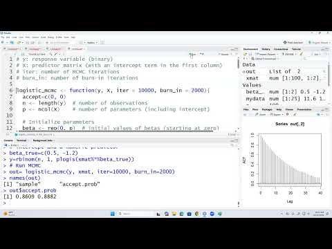
With proposal standard deviation 0.1, acceptance rates are about 0.86 and 0.88, indicating proposals are often close to the current parameter values.
Increasing the proposal standard deviation to 0.5 produces acceptance rates around 0.47 and 0.54; setting it to 0.6 gives about 0.40 and 0.47.
Sinha recommends tuning toward roughly 30% to 50% acceptance and notes that separate parameters can use different proposal scales.

7:32 Diagnosing MCMC Chains with Trace Plots, ACF, ESS, and R-hat

Use trace plots and autocorrelation function plots together: ACF lag 1 measures dependence between consecutive chain values, while trace plots reveal how parameters move over iterations.
High autocorrelation slows exploration of the joint posterior; effective sample size falls below the number of MCMC iterations as dependence increases.
Monte Carlo standard error accounts for chain dependence, while Gelman-Rubin R-hat compares within-chain and between-chain variation across multiple chains.
Diagnostics identify problems but do not resolve them; possible responses include longer runs, thinning, proposal changes, block sampling, or collapsing steps.

20:17 Checking Logistic-Regression Convergence Across Three Chains

Sinha fits the same logistic model in three chains with different initial values: (-1, 1), (1, -1), and (1, 1).
The reported R-hat estimates are 1.01 for the intercept and 1.02 for the slope, consistent with the chains approaching the same target distribution.
He describes values near 1 as favorable and values above roughly 1.10 as a warning sign; BRMS commonly defaults to 4 chains.

23:12 Replacing the Logistic Link with a Probit Model

For binary outcomes, the probit model specifies the success probability as the standard normal CDF, Φ(Xᵀβ), instead of a logistic function.
With one observed predictor Z, the linear predictor is β₀ + β₁Z, where β₀ is the intercept and β₁ is the slope.
The binary-response likelihood uses pᵢ raised to yᵢ and (1 − pᵢ) raised to 1 − yᵢ; Metropolis-Hastings uses the resulting log likelihood.
The complementary log-log link is another option for modeling binary success probabilities.

29:47 Why Block Sampling Can Improve Slow-Mixing Chains

Component-wise sampling updates one parameter at a time and can leave strongly correlated parameters with stubborn autocorrelation, even after proposal tuning.
Block sampling jointly updates a group of correlated parameters, potentially reducing autocorrelation and improving chain mixing.
Sinha cautions that block sampling is not guaranteed to solve every convergence problem, so trace plots, ACF plots, and effective sample sizes remain important.

32:01 Building a Correlated-Predictor Logistic-Regression Example

The simulation uses 500 observations and 6 design-matrix columns, including an intercept, with predictors generated to be strongly correlated.
Predictors are generated from a multivariate normal construction with unit diagonal variances and off-diagonal correlations around 0.7; the example also includes continuous and binary covariates.
Sinha constructs a logistic-regression likelihood and uses a Laplace approximation to form the covariance component of a multivariate normal block proposal.
The comparison is between component-wise random-walk Metropolis and block random-walk Metropolis.

37:37 Comparing Component-Wise and Block-Sampling Results

Trace plots for the intercept and two regression coefficients show pronounced dependence under component-wise sampling and reduced dependence under block sampling.
The component-wise ACF remains high even at lag 58, around 0.5 in the displayed example; block sampling lowers the correlations but does not eliminate them.
Posterior means from the two methods are similar in the displayed estimates, while the time-series standard error accounts for autocorrelation.
Sinha frames MCMC tuning as iterative work: inspect diagnostics, adjust proposal or block settings, and rerun the chain.

42:50 BRMS, Hamiltonian Monte Carlo, and Posterior Prediction

BRMS offers a higher-level route to Bayesian logistic regression: specify the response, predictors, and prior distributions rather than writing the sampler yourself.
The package uses Hamiltonian Monte Carlo with the No-U-Turn Sampler (NUTS), rather than the component-wise or block Metropolis methods discussed earlier.
Posterior predictive probabilities can be evaluated for new covariate values by passing new data to the fitted model and averaging the resulting probabilities.
Sinha illustrates prediction for specified predictor combinations, including values such as X₁ = −1 and X₂ = 0.

48:12 Collapsed Gibbs Sampling and Breaking Iteration-to-Iteration Dependence

Standard Gibbs sampling alternates conditional updates, such as θ₁ given θ₂ and data, then θ₂ given θ₁ and data.
Collapsed Gibbs sampling can instead draw one parameter from its marginal posterior given the data, then draw the other conditional on that new value.
Because the marginal draw need not use the previous iteration's value, collapsing can break some dependence between consecutive samples.
Sinha connects the idea to the normal model with unknown mean μ and variance σ², and notes that collapsed sampling is only applicable when the required marginal distributions are available.

Summary, takeaways, and chapters were generated by AI from the video's transcript and may contain errors. The video belongs to its creator, Samiran Sinha.