STAT 638 (Fall 2026), Lecture 27

Overview

Samiran Sinha reviews two Bayesian linear regression quiz problems: a known-variance normal model, then a model with an unknown variance and a Zellner g-prior. He derives the conditional posterior distributions, demonstrates Monte Carlo estimation with R and MASS::mvrnorm, and uses Gibbs sampling to estimate a 95% posterior predictive interval for a new outcome at x* = (1, 2), obtaining approximately [-2.32, 5.06].

Key takeaways

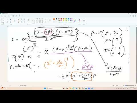
With known σ² and a normal prior, Bayesian linear regression has a normal posterior with covariance (Σ⁻¹ + XᵀX/σ²)⁻¹ and mean equal to that covariance times (Σ⁻¹μ + XᵀY/σ²).
A posterior probability such as P(β₁ > β₂ | data) can be estimated by simulating 10,000 draws from the joint posterior and calculating the fraction satisfying β₁ > β₂.
For the g = 4 prior β | σ² ~ N(0, 4σ²(XᵀX)⁻¹), the conditional posterior covariance is (σ²/1.25)(XᵀX)⁻¹ and its mean is 0.8(XᵀX)⁻¹XᵀY.
With n = 16 coefficients' observations, p = 2 regression coefficients, and π(σ²) ∝ 1/σ², the conditional inverse-gamma shape for σ² is (n + p)/2 = 9.
A posterior predictive draw must add a new observation error to x*ᵀβ; for x* = (1, 2), Gibbs-based simulation produced an approximate 95% interval of [-2.32, 5.06].

Chapters

0:00 Quiz 4, Question 1: Set Up the Gaussian Regression Model

The first problem has 16 experimental units, a 16-by-2 design matrix X without an intercept, and outcome vector Y.
Assume Y | β follows a normal distribution with mean Xβ and covariance σ²I, with σ² fixed at 2.
The prior is β ~ N(μ, Σ), where μ = (0, 1) and Σ = diag(1, 4); the target is P(β₁ > β₂ | data).

5:30 Derive the Normal Posterior Mean and Covariance

Combine the Gaussian likelihood and normal prior by collecting the quadratic and linear terms in β.
The posterior covariance is (Σ⁻¹ + XᵀX/σ²)⁻¹.
The posterior mean is the covariance multiplied by (Σ⁻¹μ + XᵀY/σ²), with matrix dimensions checked throughout.

13:30 Check the Regression Inputs and Posterior Matrix Calculations

Use the provided summary quantities XᵀX and XᵀY rather than reconstructing all 16 rows of observations.
Substitute σ² = 2 and the stated prior values into the posterior formulas to obtain a two-dimensional normal distribution.
Sinha recommends checking that the covariance matrix is 2-by-2, symmetric, and positive definite before sampling.

18:15 Estimate P(β₁ > β₂) with MASS::mvrnorm

Draw 10,000 samples from the bivariate normal posterior using the mvrnorm function in R's MASS package.
Estimate the probability by counting draws where β₁ exceeds β₂ and dividing the count by 10,000.
The reported Monte Carlo estimate is approximately 0.09; Sinha also catches an R matrix-multiplication error while checking the posterior mean.

23:45 Quiz 4, Question 2: Introduce a Zellner g-Prior

The second problem retains n = 16 and the supplied XᵀX and XᵀY, and adds YᵀY = 64.
Set β | σ² ~ N(0, gσ²(XᵀX)⁻¹) with g = 4, and use the improper variance prior π(σ²) ∝ 1/σ².
The goal is a 95% posterior predictive interval for a future outcome at a specified explanatory vector.

31:30 Derive β Conditional on σ² Under the g-Prior

The prior precision contributes (XᵀX)/(4σ²), while the likelihood precision contributes XᵀX/σ².
Combining them gives conditional posterior covariance (σ²/1.25)(XᵀX)⁻¹.
Because the prior mean is zero, the posterior mean simplifies to (1/1.25)(XᵀX)⁻¹XᵀY.

36:50 Derive the Inverse-Gamma Conditional Distribution for σ²

Given β and the data, σ² has an inverse-gamma conditional posterior with shape (n + p)/2; here n = 16 and p = 2.
Its scale combines the residual sum of squares (Y − Xβ)ᵀ(Y − Xβ) with the g-prior term βᵀXᵀXβ/4, with the combined expression divided by 2.
Sinha notes that the inverse-gamma scale corresponds to the gamma distribution's rate when sampling by taking the reciprocal of a gamma draw.

40:55 Build the Gibbs Sampler for β and σ² in R

Alternate draws from β | σ², Y and σ² | β, Y to generate samples from the joint posterior.
Compute each residual sum of squares from YᵀY − 2βᵀXᵀY + βᵀXᵀXβ, using the supplied sufficient statistics.
Initialize β and σ², calculate the conditional mean and covariance, and run repeated updates to form posterior samples.

47:45 Simulate New Outcomes at x* = (1, 2)

For each posterior draw of β and σ², generate a fresh error ε* ~ N(0, σ²).
Construct each predictive draw as Y* = x*ᵀβ + ε*, using x* = (1, 2).
Including ε* represents both uncertainty in the regression parameters and observation-level noise.

52:10 Read the Approximate 95% Posterior Predictive Interval

The simulated predictive distribution gives an approximate 95% interval from -2.32 to 5.06.
Sinha cautions that Monte Carlo output can vary between runs, so nearby answers are reasonable.
The lecture concludes by noting that AI produced correct answers for these quiz problems.

Transcript excerpt

0:00 Sinha, Samiran: Alright, let's get started. Sinha, Samiran: Today, we'll talk about wheeze? Sinha, Samiran: Quiz… quiz number 4, discussions, and then, we'll talk about the rest of the part. Sinha, Samiran: of GLM. Sinha, Samiran: And if time permits, then we'll talk about multimedia normal. Sinha, Samiran: part, which is on Chapter 7. Remember, we skipped that chapter, so after GLM, we'll come back to Chapter 7. This is the plan, I don't know whether I'll be able to start it today.

0:59 Sinha, Samiran: So, quiz 4, question number 1, suppose that we have outcome and explanatory variable data from 16 experimental units. Oh, by the way, everyone did very well in the quiz, so… but anyhow, I'll be discussing all the quiz questions. Sinha, Samiran: The outcome vector is Y, and the design matrix X is of dimension. Sinha, Samiran: The outcome vector is Y, and the design matrix X is of dimension 16 by 2 without the intercept. Sinha, Samiran: without the intercept. No intercept is there. Now, we write all the assumptions using notation, so Y given beta and sigma squared follows normal distribution. Sinha, Samiran: With the mean X beta, and variance sigma squared times the identity matrix. Sinha, Samiran: X transpose X is given, X transpose Y is given, the prior for beta.

1:58 Sinha, Samiran: is given to U, and the prior density for sigma squared. Sinha, Samiran: Is pi sigma squared proportional to 1 over sigma squared. Sinha, Samiran: What is probability, beta 1? Sinha, Samiran: greater than beta 2, given the data. Now, data means, generally, we Sinha, Samiran: Talk about Y. Y is the outcome which has noise in it, and X, the design matrix. Sinha, Samiran: is generally treated as the given quantity. So, usually, X is not part of the data, therefore I did not write it, but it does not mean that we'll not be including X.

This is the start of the transcript. Save this video free for the whole transcript, searchable and time-coded.

Related notes

Summary, takeaways, and chapters were generated by AI from the video's transcript and may contain errors. The video belongs to its creator, Samiran Sinha.