STAT 638 (Fall 2026), Lecture 24

Overview

Samiran Sinha explains Bayesian variable selection with spike-and-slab priors, then introduces Metropolis-Hastings MCMC through a Bayesian logistic regression for diabetes prediction. He covers posterior inclusion probabilities, model-selection error measures, acceptance ratios and proposal choices, and an R implementation using 10,000 iterations with a 2,000-iteration burn-in.

Key takeaways

A spike-and-slab prior represents predictor exclusion with a near-zero spike and inclusion with a broader slab, while posterior inclusion probabilities quantify evidence for each feature.
In a simulation with 100 subjects, 50 predictors, and five truly nonzero effects, spike-and-slab selection gave three true predictors inclusion probabilities above 0.5.
When predictors are standardized in logistic regression, exp(βₖ) describes the odds ratio for a one-standard-deviation increase, not necessarily a one-unit increase in the original measurement.
Metropolis-Hastings can sample from a posterior known only up to a proportionality constant by proposing candidates and correcting for proposal probabilities in the acceptance ratio.
A symmetric normal random-walk proposal cancels from the Metropolis-Hastings ratio, leaving only target-density comparisons; Sinha’s implementation uses proposal standard deviation 0.1.
Gibbs sampling is a special case of single-component Metropolis sampling in which proposals come directly from the full conditional and are accepted with probability 1.

Chapters

0:00 Bayesian Model Selection: From Marginal Likelihood to MCMC

For linear regression, marginal likelihood can compare models analytically, but evaluating many models becomes costly as the predictor count grows.
MCMC can explore models according to their posterior probabilities without computing the marginal likelihood for every model.
Model-averaging methods such as BMA and BAS estimate posterior model probabilities and predictor inclusion probabilities.

3:47 BMA and BAS for the 442-Patient Diabetes Dataset

The diabetes example has 442 patients, with disease progression one year after baseline as the outcome.
The dataset has 10 baseline covariates, expanding to 64 predictors when second-order terms are included.
Bayesian model averaging and Bayesian Adaptive Sampling (BAS) help identify important predictors when the relationship may not be linear.

5:13 Spike-and-Slab Priors Encode Predictor Inclusion

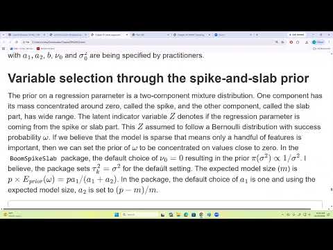
Each coefficient βₖ uses a two-component normal mixture: a spike concentrated near zero with variance 0.001² and a slab with variance τₖ².
A Bernoulli indicator Zₖ selects the spike or slab; the inclusion probability ω has a Beta prior, while slab variance and residual variance have inverse-Gamma priors.
The prior expected model size is P times E[ω]; the package default sets A₁ = 1 and chooses A₂ from the desired model size M.
The method targets parsimonious models and is useful in genomics, where thousands of gene-expression features may be measured on far fewer patients.

11:42 Simulating Spike-and-Slab Selection with 50 Predictors

Sinha simulates 100 subjects and 50 standard-normal features, with only the first five coefficients nonzero and drawn from Uniform(−1, 1).
The response is generated from Xβ plus standard-normal noise, then fitted with the R function lm.spike using default settings.
Posterior inclusion probabilities exceed 0.5 for three of the five true predictors, while other features receive lower probabilities.
The posterior for the first coefficient is bimodal, with a spike near zero and a slab on the negative side, illustrating uncertainty about inclusion.

17:51 Assessing Feature Selection with FDR, FNR, and F1

A posterior inclusion probability threshold of 0.5 can turn Bayesian inclusion estimates into selected or excluded features.
Repeated simulations measure false positives among truly unimportant predictors and false negatives among truly important predictors.
False discovery rate and false negative rate often trade off, so Sinha also recommends comparing methods using the F1 score.
Bayesian Lasso and horseshoe priors are presented as alternatives to spike-and-slab selection.

22:13 Bayesian Logistic Regression for Diabetes Prediction

The motivating model predicts diabetes among women using pregnancies, blood pressure, body mass index, diabetes pedigree, and age.
Predictors are centered and scaled; the binary outcome is modeled with probability logistic(Xᵀβ), where X includes an intercept.
Exponentiated coefficients describe conditional odds ratios, but scaling means a coefficient represents a one-standard-deviation predictor increase rather than a one-unit increase.
Bayesian inference targets posterior distributions for the regression coefficients instead of only frequentist point estimates.

28:08 Why the Logistic Posterior Requires MCMC

Independent Bernoulli observations yield a likelihood formed from each subject’s logistic success probability and observed 0/1 outcome.
Normal priors for the logistic coefficients combine with the likelihood to define the posterior distribution.
The resulting full conditional distributions do not have convenient forms for direct sampling, motivating general MCMC methods.
Posterior samples support estimates such as coefficient means and credible intervals.

34:25 Metropolis-Hastings Acceptance Ratios and Proposal Choices

Metropolis-Hastings proposes a candidate from an easy-to-sample distribution, then accepts it with probability min(1, R); otherwise it retains the current value.
The acceptance ratio R adjusts the target-density ratio by the forward and reverse proposal densities.
A symmetric proposal, such as a normal random walk centered at the current value, cancels the proposal terms and gives the Metropolis algorithm.
An independent proposal does not depend on the current state; it works well when it closely matches the target density, and performs poorly when the match is weak.

40:57 Single-Component Metropolis Updates and Gibbs Sampling

Single-component Metropolis updates change one coordinate of a parameter vector at a time, targeting that coordinate’s conditional distribution given the rest.
The target density need only be known up to a proportionality constant, which is important when posterior normalizing constants are unavailable.
Gibbs sampling is a special case: if the proposal equals the full conditional distribution, the acceptance probability is 1.
A mixed algorithm can use direct Gibbs draws for tractable conditionals and Metropolis-Hastings for conditionals known only up to a constant.

44:38 Implementing Logistic MCMC with a Normal Random-Walk Proposal

The R example runs 10,000 iterations, discards the first 2,000 as burn-in, and initializes regression coefficients at zero.
Each coefficient is proposed from a normal distribution centered at its previous value with standard deviation 0.1.
Because this random-walk proposal is symmetric, the acceptance calculation uses the proposed-versus-current log likelihood plus log prior, avoiding unstable raw likelihood products.
Sinha cautions against extreme initial values that can overflow exponential terms; convergence diagnostics and sampling results are deferred to the next lecture.

Summary, takeaways, and chapters were generated by AI from the video's transcript and may contain errors. The video belongs to its creator, Samiran Sinha.