Math317Fa26 Lec23 MathematicalModelingDiscrete Roulette
 Watch on YouTube →
Overview
Steven Miller connects probability and difference equations to mathematical modeling, using an age-structured whale population and matrix methods to show how discrete systems can be analyzed. He then examines roulette’s double-plus-one betting strategy: although it appears profitable in an ideal 50/50 game with unlimited funds, table limits make losing streaks dangerous, and a recurrence estimates an 81% chance of five consecutive blacks within 100 spins.
Key takeaways
- The double-plus-one strategy does not remove roulette risk: after a sequence of losses, the required bet grows exponentially, and table limits can prevent the next recovery bet.
- In a fair 50/50 roulette model, the chance of encountering five consecutive blacks is about 81% within 100 spins and 96.59% within 200 spins.
- An age-structured population model becomes a linear discrete system when its age classes and birth rules are explicit; a fixed 4×4 transition matrix advances the population one year at a time.
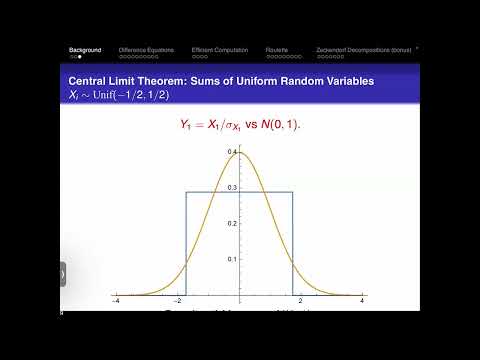
- For independent, identically distributed random variables, centering and scaling their sum by σ√n leads to an approximate standard normal distribution, often simplifying calculations.
- Historical roulette results provide no predictive advantage when spins are independent: a color streak does not make that color more likely or make the other color 'due'.
- Mathematical models depend on assumptions: unlimited funds and a fair roulette wheel create an idealized setting, while table limits, finite resources, and green pockets change the real-world outcome.
Chapters
- A probability density is nonnegative, integrates to 1, and assigns probabilities through areas under its curve.
- The mean weights possible values by probability; variance measures squared spread, while standard deviation returns spread to the original units.
- Independence means learning one random variable gives no information about another; Miller cautions that hidden dependencies can be easy to miss.
- The spelling and foot-size example illustrates confounding: older children may have both larger feet and better spelling, so correlation does not establish causation.
- A normal distribution is specified by mean μ and variance σ², with its density normalized by √(2πσ²).
- For independent, identically distributed variables with finite mean and variance, the centered sum divided by σ√n approaches a standard normal distribution.
- The sum of two fair six-sided die rolls has a triangular distribution, while sums of four and eight normalized uniform variables look progressively more normal.
- The central limit theorem replaces complicated piecewise distributions with a useful normal approximation.
- A difference equation defines a sequence from earlier values, making it the discrete-time counterpart of a differential equation.
- The Fibonacci recurrence uses the previous two terms, and matrix powers can compute distant terms far more efficiently than stepping through every value.
- Constant-coefficient recurrences can often be solved through eigenvalues, although general polynomial equations of degree five or higher lack radical formulas.
- Miller models whale pairs in four age classes: newborns Aₙ, one-year-olds Bₙ, two-year-olds Cₙ, and three-year-olds Dₙ.
- The assumptions make each one-year-old pair produce two pairs and each two-year-old pair produce one; whales age into the next class and die at four.
- The population update is deterministic and can be written as a fixed 4×4 matrix multiplied by the age-count vector, then iterated with matrix powers.
- The model omits random births, variable lifespans, and finite resources; predator-prey questions show how resource limits can change population outcomes.
- Real population transitions may require random matrices rather than the whale model’s fixed update matrix.
- The matrix exponential is defined by the power series for eˣ with a square matrix substituted, and the series converges for every square matrix.
- In general, eᴬeᴮ is not eᴬ⁺ᴮ because matrix multiplication may not commute; the commutator AB − BA measures the failure to commute.
- The Baker-Campbell-Hausdorff formula expresses the product through additional nested commutator terms.
- Standard American roulette has 18 red pockets, 18 black pockets, and green 0 and 00; Miller first removes both greens to create an idealized 50/50 game.
- The double-plus-one strategy starts with a $1 bet on red and doubles after each loss: bets of $1, $2, $4, and $8 recover prior losses and net $1 if a later bet wins.
- The strategy appears to guarantee eventual profit only if the gambler can keep increasing the bet indefinitely and has unlimited funds.
- A finite table maximum blocks the doubling sequence: after losing $1, $2, $4, $8, $16, and $32, the next desired bet is $64.
- With a $50 table maximum, the gambler cannot place the required $64 bet and remains $63 down, so even a $50 win leaves a net loss.
- Past roulette outcomes do not predict future spins when spins are independent; both betting on a streak and believing the opposite color is due are mistaken heuristics.
- Casinos may benefit when players experience small wins before a rare, large loss, since visible short-term success encourages more play.
- Let Pₙ be the probability of avoiding five consecutive blacks in n fair spins; conditioning on an initial red or a run of blacks yields a recurrence using the previous five values.
- The initial probabilities P₀ through P₄ are all 1, and the recurrence gives P₅ = 31/32, matching the chance that five spins are not all black.
- The probability of at least one five-black streak reaches 81% within 100 spins and 96.59% within 200 spins.
- These streak probabilities quantify why a finite bankroll or table limit makes the doubling strategy vulnerable even in a fair game.
- A casino can treat the table maximum as a design parameter, balancing player bankrolls, willingness to continue, and the frequency of apparent small wins against large losses.
- A more realistic analysis restores 0 and 00, making a red bet less likely to win than in the idealized 50/50 model and increasing the risk of a losing streak.
- Miller contrasts doubling to recover a fixed $1 with questions raised by the Kelly criterion about how much to wager.
- Simulations illustrate the strategy’s risk profile: a player can appear to do well for many spins, then lose heavily when an unlucky streak arrives.
Transcript excerpt
0:00 to math 317 operations research. So, what I want to do now is I want to, you know, continue to talk about places where you can use operations research, places where you can try to figure out what is the optimal strategy, what is the best thing to do. There's lots of different places we can ask stuff like this. So, I thought I would talk a little bit about mathematical modeling. This is also, as I've been saying, a good time to give a little shout out to what classes you might want to take next semester. So, I'll be doing probability, Professor Blackwood will be doing mathematical biology where they will be doing a lot of modeling in a class like this. I'm going to start by doing discrete systems today, and then on Monday we will shift to continuous systems. I have been told that there are things in the world other than sports. I'm not entirely convinced of this, but I have been told, so I will have examples from
0:47 outside of sports. On Monday we will do things from naval warfare, from the Battle of Trafalgar. Okay. So, we're going to quickly review some basic probability. I'll assume by now most people have a rough idea of the real basics of probability. We're not going to need too much. I want to talk a little bit about difference equations. You've probably seen difference equations before. These are the discrete versions of differential equations. Differential equations are a lot nicer for many things because we have calculus. You've spent three semesters taking calculus classes. It would be nice to be able to use that material to do something. We'll talk about how to solve different types of difference equations. And I don't believe we've analyzed roulette in
This is the start of the transcript. Save this video free for the whole transcript, searchable and time-coded.
In this course
Related notes
Summary, takeaways, and chapters were generated by AI from the video's transcript and may contain errors. The video belongs to its creator, Steven Miller.