Math317Fa26 Lec7 EuclideanAlgorithmFundamentalTheoremOfCalculus
 Watch on YouTube →
Overview
Steven Miller uses the Euclidean algorithm and the Fundamental Theorem of Calculus to show how algorithm analysis and mathematical proofs can rely on bounds rather than exact computation. The Euclidean algorithm preserves the GCD while its remainders shrink geometrically, giving logarithmic runtime; the calculus proof traps area between upper and lower sums, then uses the Mean Value Theorem and a telescoping sum to identify it as F(b) − F(a).
Key takeaways
- The Euclidean algorithm preserves the GCD because gcd(x, y) = gcd(x, y − ax), allowing repeated division to reach the answer constructively.
- Euclidean remainders decrease by at least a factor of 2 every two steps, so the number of divisions grows logarithmically with the input's numeric size rather than linearly.
- Reversing the Euclidean division equations produces Bézout coefficients, expressing gcd(x, y) as αx + βy.
- For a function with bounded derivative on [0, 1], the gap between upper and lower sums is at most sup|f′|/n, so the two bounds converge to the same area.
- Applying the Mean Value Theorem to an antiderivative on each partition interval makes the sum telescope to F(1) − F(0), proving the area formula.
- Optimization often needs a sufficiently tight feasible lower and upper bound rather than an exact answer, especially when computation must finish within a fixed deadline.
Chapters
- Miller distinguishes average runtime from worst-case runtime, since different inputs can require different numbers of calculations.
- The right optimization target depends on the task: a Lego Star Destroyer build needed to finish in under 10 minutes, not to minimize every builder's time.
- An algorithm that is acceptable for a one-time calculation may be unsuitable when repeated or when a hard deadline applies.
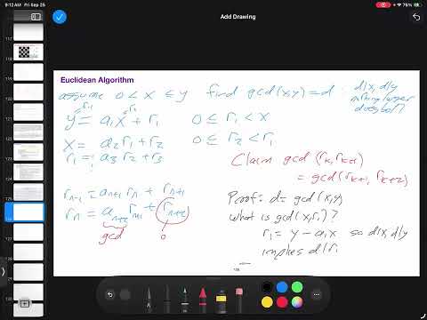
- For positive integers 0 < x ≤ y, divide y by x and write y = a₁x + r₁, with 0 ≤ r₁ < x.
- Continue dividing each remainder by the one before it; the remainders strictly decrease until one is zero.
- The last nonzero remainder is the greatest common divisor, so the procedure constructs a GCD rather than merely asserting that one exists.
- Because r₁ = y − a₁x, every common divisor of x and y also divides r₁.
- Conversely, a common divisor of x and r₁ divides y = a₁x + r₁, so gcd(x, y) = gcd(x, r₁).
- Repeating this equality down the remainder sequence proves the final nonzero remainder is the original GCD.
- Reversing the division equations also yields Bézout coefficients α and β such that gcd(x, y) = αx + βy.
- A crude worst-case argument allows each remainder to decrease by only 1, suggesting as many as x steps.
- For values near 10^400, that numeric bound is infeasible, but it assumes the worst possible decrease at every step.
- Miller reframes the analysis by showing that the sequence must shrink substantially over pairs of divisions.
- For consecutive remainders, either the next remainder is already at most half the previous one, or it is greater than half.
- In the second case, the quotient at the next division must be 1, so the following remainder is the difference of the two remainders and is less than half.
- Thus every two Euclidean steps reduce the remainder by at least a factor of 2, establishing logarithmic rather than linear growth in the input value.
- Miller connects fast GCD computation to RSA encryption, where numbers around 10^400 may be involved.
- The geometric decrease implies a number of divisions proportional to log₂ x; the lecture uses roughly 1,600 steps as a classroom-scale estimate for a 10^400 input.
- The worst-case bound may differ substantially from typical behavior, so Miller raises average-case analysis and especially good or bad inputs as further questions.
- A movie-theater scheduling application illustrates deadline-driven optimization: results had to be ready within a two-hour newspaper printing window, even if they were not provably optimal.
- For a suitable function f with antiderivative F, the theorem identifies the area under f from a to b as F(b) − F(a).
- Miller emphasizes that the theorem is about area, not just the formula for evaluating an integral.
- The proof assumes a bounded interval and continuous derivatives, and uses the Mean Value Theorem: average change equals an instantaneous derivative at some point.
- The speed analogy explains the theorem: if average speed is 40 miles per hour, continuity ensures the instantaneous speed reaches 40 at some time.
- Partition [0, 1] into n intervals of width 1/n and choose each interval's minimum and maximum function values.
- A rectangle using the minimum gives a lower estimate of the area, while one using the maximum gives an upper estimate.
- Summing the rectangles produces lower and upper sums that trap the true area between them.
- On each subinterval, apply the Mean Value Theorem to the minimum and maximum points to bound their function-value difference by sup|f′| times their distance.
- Those points are at most 1/n apart, and there are n intervals, so the total upper-minus-lower gap is at most sup|f′|/n.
- If f′ is bounded, the gap tends to zero as n grows, forcing the upper and lower sums to converge to the same area.
- Choose a point xₖ in each subinterval using the Mean Value Theorem for F, so F((k+1)/n) − F(k/n) = f(xₖ)/n.
- The sum of these differences telescopes to F(1) − F(0), while the sampled sum remains between the lower and upper sums.
- As the bounds converge to the area, F(1) − F(0) equals that area; the interval can be generalized from [0, 1] to [a, b].
- Miller checks the result against f(x) = 1 and f(x) = x, then connects bounding the answer to duality in optimization: a sufficiently tight lower and upper bound can be more useful than an exact solution.
Transcript excerpt
0:00 to math 317 operations research. This is lecture seven on the uklidian algorithm fundamental theme of calculus. We have a few people who are battling bugs and are uh you're taking the class today either asynchronously or by zoom. Uh I don't see them in the zoom waiting room right now. If you do see somebody trying to join in, please just let me know. This is a little bit of a non-standard topic for an operations research class. So the reason I want to talk about these is not because of the beauty of the uklidian algorithm and the fundamental them of calculus which they're both of course beautiful wonderful results but because it gives me a good way to talk about some of the key things we care about namely trying to determine how efficient is some algorithm how close are we to a solution that's the skill that you are going to want to really
0:47 master it is much easier for me to do it with these examples than for some of the big theorems in operations research so rather than you know having everybody do a crash course and analysis over the weekend, which again, if you are game, I'm game. Let's take something that's a lot more accessible and just go through the thought process of how do you analyze an algorithm and what do you really care about? So, when you're concerned with runtime, I know we got a couple people here who are doing CS, what do you care about when you're trying to minimize runtime? What does that mean to you? The >> the growth of the runtime. >> So, okay. So, one is the growth of the runtime, but but which runtime are you caring about? space and also space time and like how
This is the start of the transcript. Save this video free for the whole transcript, searchable and time-coded.
In this course
Related notes
Summary, takeaways, and chapters were generated by AI from the video's transcript and may contain errors. The video belongs to its creator, Steven Miller.