Math317Fa26 Lec05 SolvingPolyMatrixForms CanonicalLinProgProblem
 Watch on YouTube →
Overview
Steven Miller develops canonical forms as a way to turn unfamiliar problems into standard ones, reviewing quadratic equations, matrix diagonalization, and Jordan form before applying the idea to linear programming. He shows how to convert an optimization problem to minimizing cᵀx subject to Ax = b and x ≥ 0, then uses a diet example to explain why an optimum can be found by checking feasible-region vertices.
Key takeaways
- A quadratic can be solved by matching coefficients after rewriting it in vertex form, which produces the quadratic formula from a simpler square-root problem.
- For a diagonalizable matrix A = QΛQᵀ, high powers reduce to Aᵐ = QΛᵐQᵀ, making diagonalization useful for repeated transitions and other iterative processes.
- A Markov transition matrix with columns summing to 1 has eigenvalue 1; in the California–Florida example, trace 1.7 implies the second eigenvalue is 0.7.
- A general linear program can be converted to minimize cᵀx subject to Ax = b and x ≥ 0 by negating maximization objectives, splitting free variables as u − v, and adding or subtracting nonnegative slack variables.
- For the diet constraints 30x₁ + 5x₂ ≥ 60 and 15x₁ + 10x₂ ≥ 70, minimizing 2x₁ + 3x₂ only requires comparing the three feasible-region vertices.
- Canonical form is useful for general proofs and standardized methods, but transformations such as splitting free variables can add complexity and may be inefficient for a particular problem.
Chapters
- Steven Miller frames canonical forms as standard representations that make a problem easier to solve, much like choosing coordinates aligned with an ellipse.
- The lecture connects finding a feasible solution with choosing the best one, such as selecting among algorithms with different runtimes.
- The opening polynomial examples begin with solving ax + b = 0 when a is nonzero.
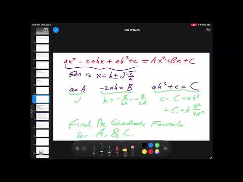
- The form a(x − h)² + c = 0 is easy to solve by isolating the square and taking square roots.
- Expanding a(x − h)² + c and matching coefficients with Ax² + Bx + C yields relations among a, h, c and A, B, C.
- This coefficient-matching method derives the quadratic formula from a simpler form rather than treating it as an isolated rule.
- A general cubic can be simplified by dividing through by its nonzero leading coefficient and shifting the variable to eliminate the quadratic term.
- Miller notes that cubic and quartic equations have general solution formulas, though their expressions become cumbersome.
- For general polynomials of degree five or higher, no formula using radicals gives all roots; numerical methods are used to approximate solutions.
- For a real symmetric matrix A, an orthogonal matrix Q gives a diagonal representation, with QᵀAQ = Λ.
- Writing A = QΛQᵀ makes powers straightforward: Aᵐ = QΛᵐQᵀ, and powers of a diagonal matrix are computed entry by entry.
- Changing coordinates can simplify a transformation, just as rotating axes to align with an ellipse makes its geometry easier to describe.
- A two-state California–Florida model uses transition probabilities 0.8 and 0.9 for residents staying, with 0.2 and 0.1 moving between states.
- The transition matrix has columns summing to 1, so 1 is an eigenvalue; its trace is 1.7, giving the other eigenvalue as 0.7.
- When diagonalization is unavailable, a matrix can be put into upper-triangular or Jordan form by a change of coordinates.
- Jordan blocks place an eigenvalue along the diagonal and ones immediately above it, providing a structured alternative to diagonal form.
- The target form is to minimize cᵀx subject to Ax = b and x ≥ 0.
- Using one standard form helps make problems easier to handle systematically and reduces the chance of inconsistent setup.
- The three features to normalize are the objective direction, variable signs, and constraint equalities.
- Maximizing cᵀx is equivalent to minimizing −cᵀx over the same feasible set.
- The transformation uses the additive inverse of the coefficient vector, not a reciprocal or matrix inverse.
- This conversion lets a solver designed for minimization handle a maximization problem without changing its constraints.
- Any unrestricted variable x can be represented as u − v, where u and v are both nonnegative.
- The representation allows a canonical nonnegative-variable formulation but increases the number of variables and can make a particular problem harder.
- For an inequality such as aᵢᵀx ≤ bᵢ, a nonnegative slack variable fills the gap; for aᵢᵀx ≥ bᵢ, a nonnegative variable is subtracted.
- These transformations establish the standard form without implying that it is always the most efficient formulation for computation.
- The example chooses quantities x₁ and x₂ of two foods, with requirements 30x₁ + 5x₂ ≥ 60 and 15x₁ + 10x₂ ≥ 70.
- The restrictions x₁ ≥ 0 and x₂ ≥ 0 confine candidate diets to the first quadrant.
- Each nutrient requirement defines a half-plane; testing (0, 0) identifies the side that fails the requirement, so the feasible region lies on the opposite side.
- The two constraint lines and the coordinate axes define three relevant corner points of the feasible region.
- With costs of 2 per unit of x₁ and 3 per unit of x₂, equal-cost combinations lie on lines 2x₁ + 3x₂ = constant, each with negative slope.
- Sliding an equal-cost line toward lower values reaches the feasible-region boundary; continuing along it leads to a boundary corner with no greater cost.
- An optimum therefore occurs at a vertex, though a whole edge can tie if its slope matches the cost line.
- Checking the three feasible vertices replaces examining infinitely many possible diets with a finite comparison.
Transcript excerpt
0:01 Okay, welcome to math 317, operations research. This is lecture five and we're going to be talking today about canonical forms. So I'm just trying to see if it is showing that it's recording on the screen. It looks like it. All right. So what I want to do today is talk about things that you have seen a long time ago. So long ago, you probably don't even remember when you first learned how to do this. Solving polomials. And the idea is one of the big things we do in mathematics is we solve equations. We find the solutions. If there's only one solution, then we're out of luck. That's what we have to work with. But frequently in life, you will have multiple solutions and you want to then determine which of the many solutions is best for the purpose you have at mind. Uh some of you have been talking with me before class about computer science problems where you have
0:48 many different algorithms that will work and solve the problem, but the runtime could be very different. And so you might be concerned with first I wanted to be able to solve the damn problem and then once I can solve it I want to solve it efficiently. I want to minimize time and that's what we're going to be leading up to. I'll talk a little bit about diagonalizing matrices just to get a sense of what you have seen. This is leading to our discussion of canonical form is that frequently when you are looking at a problem the goal is to convert it to something you've seen before. So can you somehow convert something to a configuration that reminds you ah I know how to do this. There's many different ways of
This is the start of the transcript. Save this video free for the whole transcript, searchable and time-coded.
In this course
Related notes
Summary, takeaways, and chapters were generated by AI from the video's transcript and may contain errors. The video belongs to its creator, Steven Miller.