Lecture 2b
Overview
The lecture derives the multiple linear regression least-squares solution by differentiating the residual sum of squares (RSS), rewriting the gradient with matrix operations, and obtaining the normal equations. It then introduces sample means, variances, covariance matrices, and cross-covariance vectors as interpretable summaries of the data, deriving equivalent formulas that prepare for expressing regression coefficients through these statistics.
Key takeaways
- For a design matrix A containing a column of ones for the intercept, least squares satisfies AᵀAβ̂ = Aᵀy and, when AᵀA is invertible, β̂ = (AᵀA)⁻¹Aᵀy.
- AᵀA is invertible only when the columns of A are linearly independent; having more coefficients than training samples is one situation that prevents a unique inverse-based solution.
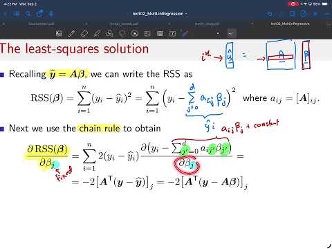
- The gradient of RSS with respect to β is −2Aᵀ(y − Aβ), so minimizing squared residuals reduces to setting a matrix-vector expression equal to zero.
- With division by n, feature covariance matrix diagonal entries are sample variances and off-diagonal entries measure pairwise feature covariance.
- The feature-target cross-covariance vector collects one covariance per feature, and its raw-moment form is (1/n)∑ᵢ xᵢyᵢ − x̄ȳ.
- Sample variance uses squared units, while sample standard deviation takes its square root to return to the units of the original feature or target.
Chapters
- The prediction combines features with coefficients and an intercept: for two features, β₀ sets the plane's height and β₁ and β₂ set its slopes.
- The residual εᵢ is the difference between predicted and observed target values for sample i.
- Least squares selects the coefficients that minimize the sum of squared residuals across the training samples.
- The RSS is the squared Euclidean norm of the target vector minus the predicted-target vector.
- At the minimum of the RSS bowl, the slope with respect to every coefficient is zero.
- The vector of partial derivatives is the gradient, so the least-squares solution satisfies a zero-gradient condition.
- The prediction for sample i is the row-feature sum ∑ⱼ Aᵢⱼβⱼ, including the intercept column in A.
- Applying the chain rule to each squared residual produces a factor of 2 and the derivative of the prediction.
- When differentiating with respect to βⱼ, all terms involving other coefficients are constant; only Aᵢⱼβⱼ contributes, while the observed target yᵢ has derivative zero.
- The derivative for coefficient βⱼ sums the residuals weighted by the corresponding feature values Aᵢⱼ.
- Stacking those weighted residual sums across coefficients gives the vector Aᵀ(y − ŷ).
- Substituting ŷ = Aβ converts the expression to Aᵀ(y − Aβ), with the overall factor −2 omitted when setting the gradient to zero.
- Setting the gradient to zero yields Aᵀy = AᵀAβ.
- If AᵀA is invertible, the coefficient estimate is β̂ = (AᵀA)⁻¹Aᵀy.
- In practice, assemble A from the training features plus a column of ones, place targets in y, and use a numerical package such as NumPy to solve for the coefficients.
- The inverse fails when the design matrix lacks full column rank; having more coefficients than samples is one concrete case.
- The predictor can be written as β₀ + β₁:dᵀx, separating the intercept from the feature slopes.
- The target sample mean is ȳ = (1/n)∑ᵢ yᵢ, and the mean of feature j is x̄ⱼ = (1/n)∑ᵢ xᵢⱼ.
- These sample means are deterministic averages of the observed training data, distinct from population means of random variables.
- The lecture defines sample variance as the average squared deviation from the sample mean, dividing by n for this derivation.
- Taking the square root gives sample standard deviation, which has the same units as the original data, unlike variance.
- Sample covariance averages the product of deviations for a feature and the target, capturing how they vary together.
- Dividing by n − 1 is a convention used in other settings, but the formulas here require division by exactly n.
- Averaging each training feature vector across samples gives the feature mean vector x̄, whose entries are x̄₁ through x̄ᴅ.
- The sample autocovariance matrix averages the outer products (xᵢ − x̄)(xᵢ − x̄)ᵀ.
- Diagonal entry j,j is the variance of feature j; off-diagonal entry j,k is the covariance between features j and k.
- The lecture distinguishes xᵢ, a training sample, from x, a feature vector that may be supplied later for prediction.
- Averaging (xᵢ − x̄)(yᵢ − ȳ) produces a length-d sample cross-covariance vector.
- Its jth entry is the covariance between feature j and target y, extending the scalar feature-target covariance to all features.
- Together, feature autocovariance and feature-target cross-covariance summarize relationships needed to interpret regression coefficients.
- Expanding the centered outer product gives Sₓₓ = (1/n)∑ᵢ xᵢxᵢᵀ − x̄x̄ᵀ.
- Expanding the centered feature-target product gives sₓᵧ = (1/n)∑ᵢ xᵢyᵢ − x̄ȳ.
- The raw-moment forms follow by linearity of averaging and cancellation of terms, and are convenient in algebraic derivations.
- The lecture notes that the bars on x̄ and ȳ must remain in the mean-product terms.
- The Friday midterm is scheduled for the second half of lecture, with no electronic devices or note sheets and content resembling the practice exam and homework.
- Equivalent transpose forms are acceptable; students do not need to provide both versions of an answer.
- For a noninvertible AᵀA, having more coefficients to estimate than data samples is one case where a unique solution cannot be recovered by the inverse formula.
- Prof. Schniter recommends office hours and revisiting lecture material while working through homework, when gaps in understanding become clearer.
- Prof. Schniter identifies office hours and TA sessions as ways to work through specific points that block understanding.
- He notes that students often assemble the lecture's ideas during homework rather than following every derivation in real time.
- Rewatching a relevant lecture section after attempting homework can clarify details not captured in written notes.
Transcript excerpt
0:02 Okay, let's get started. >> So, we've been talking about um multiple linear regression and last time we kind of set up the method like this. So, these XI variables are the features that we're using to predict Yi. Yi is the I sample of the target in our data set. These are um the I sample of the features in our data set. And what we're doing is we are coming up with a linear combination of those features. And then we're adding this intercept term to form our estimate or prediction of yi. We're going to call that yi hat.
0:56 [clears throat] And the method that we use to choose these beta coefficients is we choose them to minimize the uh RSS residual sum of squares which is this. And so what we have here is we have the difference between our prediction and the truth for the E sample. We're going to call that epsilon I. We square that and then we sum that over all the samples in our training set [clears throat] and we choose the beta coefficients to minimize RSS. And we have this visualization which would be in the case of two different features actually just one
1:46 um I guess. is how do I want to say this? We have um so yeah sorry okay we have here two features X1 and X2 we're using for prediction we're trying to predict Y um these black dots are our data samples and we are using this linear prediction which means we are forming a plane that we use for prediction uh where given any x1 and x2 we can look up a point on this plane and that the height of that point gives us the prediction of y and [clears throat] the difference between our prediction which
This is the start of the transcript. Save this video free for the whole transcript, searchable and time-coded.
In this course
Related notes
Summary, takeaways, and chapters were generated by AI from the video's transcript and may contain errors. The video belongs to its creator, Prof. Schniter.