Lecture 2c
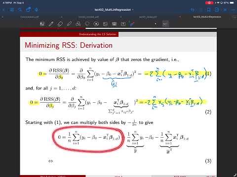 Watch on YouTube →
Overview
Least-squares regression coefficients can be expressed using dataset statistics: the feature mean, target mean, feature covariance matrix, and feature-target cross-covariance. For D features, the slope vector is SXX⁻¹SXY and the intercept is ȳ − x̄ᵀβ; the lecture then interprets the single-feature case and introduces R² as a scale-normalized goodness-of-fit measure.
Key takeaways
- For D-feature least-squares regression, the optimal slopes satisfy β = SXX⁻¹SXY, connecting feature-target covariance to feature-feature covariance.
- The optimal intercept is β₀ = ȳ − x̄ᵀβ, so the fitted predictions are centered around the target mean when evaluated at the mean feature vector.
- A single-feature least-squares slope is the feature-target covariance divided by the feature variance, SXY/SXX.
- Centering every feature and the target to mean zero makes the least-squares intercept zero.
- R² compares residual error against target variability: it equals 1 for a perfect training fit and 0 when the fit is no better than predicting the target mean.
- An invertible feature covariance matrix is required for the formula SXX⁻¹SXY; having more samples than features does not by itself ensure invertibility.
Chapters
- The derivation separates the intercept β₀ from the D slope coefficients β₁ through βD.
- The sample mean averages n observations; sample variance averages squared deviations from the mean, and covariance measures how two variables change together.
- For feature vectors Xᵢ, the sample autocovariance matrix SXX has feature variances on its diagonal and feature-to-feature covariances off the diagonal.
- The sample cross-covariance vector SXY summarizes covariance between each feature and the target Y.
- Differentiating RSS with respect to β₀ applies the chain rule to each squared residual and gives a factor of −1 from the intercept.
- Setting the intercept derivative to zero and averaging over n samples yields β₀ = ȳ − x̄ᵀβ.
- The intercept centers the fitted linear function so its predictions align with the target mean, given the slope vector.
- The intercept expression depends on β₁ through βD, so the slopes must be derived before β₀ can be evaluated.
- Differentiating RSS with respect to feature coefficient βⱼ produces a term involving Xᵢⱼ, since that feature multiplies βⱼ in each prediction.
- Substituting the intercept expression into the slope equations and collecting all feature-indexed equations gives SXY − SXXβ = 0.
- Rearranging and multiplying from the left by SXX⁻¹ gives the slope solution β = SXX⁻¹SXY.
- The inverse requires SXX to be invertible, which depends on the feature data having sufficient independent variation; having n greater than D alone does not guarantee this.
- The full coefficient vector places β₀ above the D slopes, with slopes determined by SXX⁻¹SXY and intercept by ȳ − x̄ᵀβ.
- For a single feature, the slope reduces to SXY/SXX, and the intercept reduces to ȳ − x̄(SXY/SXX).
- When both feature and target means are zero, the intercept is zero, so mean-centering during preprocessing can eliminate the need to compute it separately.
- In the single-feature case, the feature covariance matrix becomes the feature variance and the cross-covariance vector becomes a scalar covariance.
- Raw RSS grows with sample count and scales with the square of target magnitude, so it is difficult to compare across datasets.
- Dividing RSS by n removes sample-count scaling, while normalizing by the variance of Y also accounts for the target scale.
- R² is defined as one minus normalized residual error; a perfect fit has RSS = 0 and R² = 1.
- For least squares with an intercept on the training data, R² = 0 corresponds to the baseline predictor that always outputs ȳ; R² can be negative for other predictors or out-of-sample evaluations.
Transcript excerpt
0:01 All right, let's get started. So, what we did last time was we derived an expression for the least squares prediction coefficients. >> [clears throat] >> And while this expression is true, um it's not very insightful because it doesn't really clarify how like the main properties of the data set are going to affect those prediction coefficients. So, [clears throat] what we did what we started to do is um >> [clears throat] >> is re-derive the this expression um in a more interpretable way. And for this, we needed to split out the intercept coefficient in this vector from all the remaining coefficients in the vector,
0:48 which we will call beta 1 through D. So, that starts with beta 1 and goes through beta D. >> [clears throat] >> Okay. Um and then we did a a brief review of some of basic statistics, basically things like the sample mean of a list of numbers, which we will write using the overbar, and the sample variance of a list of numbers, which is [clears throat] the average squared deviation from the mean, and then the sample covariance between two lists of numbers, which tells you about some kind of like correlation of them, um how changes in one affect changes in the other.
1:35 And then we proceeded to extend these uh statistics to vectors. So, we have a sample mean vector, which is just in this case XI is the ith um sample in our data set, a vector that contains all the features for the ith sample. And so, if we average all of like that um sequence of vectors, we get the sample mean vector, bold face X bar. >> [clears throat] >> We have the sample auto covariance matrix, which is like a generalization of the variance. And so
This is the start of the transcript. Save this video free for the whole transcript, searchable and time-coded.
In this course
Related notes
Summary, takeaways, and chapters were generated by AI from the video's transcript and may contain errors. The video belongs to its creator, Prof. Schniter.