Lecture 1b
Overview
Prof. Schniter reviews the linear algebra tools used throughout the course, covering special matrices, vector norms, trace, inverses, determinants, eigenvalues, and positive-definite matrices. He then demonstrates index-based matrix “gymnastics” for turning sums into products such as CᵀB, and points students to NumPy and the first lab for computational practice.
Key takeaways
- Orthogonal matrices preserve vector length because QᵀQ = I, so multiplying by Q rotates or reflects vectors without stretching them.
- The determinant is the signed volume spanned by a matrix’s columns; determinant zero signals collapsed volume and a non-invertible matrix.
- For real symmetric matrices, orthogonal diagonalization gives A = VΛVᵀ, and A is invertible exactly when its eigenvalues are all nonzero.
- Positive definiteness can be checked through eigenvalues: a symmetric matrix with strictly positive eigenvalues makes xᵀAx positive for every nonzero x.
- To convert an indexed sum such as Σᵢ CᵢₖBᵢⱼ into matrix notation, align the summed index with the inner product dimension; the result is (CᵀB)ₖⱼ.
- The sum Σₖ[(CᵀB)ₖⱼ]² is the jth diagonal entry of (BᵀC)(CᵀB), illustrating how repeated sums become matrix products.
Chapters
- A diagonal matrix has nonzero entries only on its main diagonal; diag notation lists those entries.
- The identity matrix I has ones on the diagonal and leaves a matrix unchanged when multiplied on either side.
- A symmetric matrix satisfies A = Aᵀ, so its entries reflect across the main diagonal.
- An orthogonal matrix has mutually orthonormal rows and columns, giving QᵀQ = QQᵀ = I.
- The L2 norm is the square root of the sum of squared entries and measures ordinary Euclidean distance.
- The L1 norm sums absolute values and models Manhattan-style travel along perpendicular streets.
- Multiplication by an orthogonal matrix preserves a vector’s length, corresponding to rotation or reflection without stretching.
- The trace of an N × N matrix is the sum of its N diagonal entries.
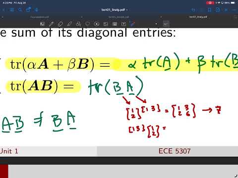
- Trace is linear: tr(αA + βB) = α tr(A) + β tr(B) for scalars α and β.
- Although AB generally differs from BA, tr(AB) = tr(BA) when the products are defined.
- For the example vectors [1, 2]ᵀ and [1, 3]ᵀ, both the outer-product trace and inner product equal 7.
- A trace requires its argument to be square, but A and B individually need not be square if AB and BA are square.
- A square matrix A is invertible when A A⁻¹ = A⁻¹ A = I; matrices without an inverse are singular.
- The inverse of an inverse returns the original matrix, and (AB)⁻¹ = B⁻¹A⁻¹ reverses product order.
- The transpose and inverse commute as operations: (A⁻¹)ᵀ = (Aᵀ)⁻¹.
- For a 2 × 2 matrix, the inverse formula swaps the diagonal entries, negates the off-diagonal entries, and divides by the determinant.
- For a 2 × 2 matrix, its columns span a parallelogram; the determinant is the signed area of that set.
- In 3D, the corresponding column combinations form a parallelepiped, whose signed volume is the determinant.
- Collinear columns collapse the spanned volume to zero, so det(A) = 0 exactly when A is non-invertible.
- For an n × n matrix, scaling the matrix by c scales its determinant by cⁿ.
- An eigenvector vᵢ keeps its direction under multiplication by A: Avᵢ = λᵢvᵢ, where λᵢ is its eigenvalue.
- Putting eigenvectors into the columns of V and eigenvalues onto the diagonal of Λ gives AV = VΛ.
- When V is invertible, rearranging gives A = VΛV⁻¹.
- The eigenvector equation describes special directions that a matrix scales rather than redirecting.
- The trace equals the sum of a square matrix’s eigenvalues, while its determinant equals their product.
- A zero eigenvalue makes the determinant zero and the matrix non-invertible.
- For a real symmetric matrix, eigenvalues are real and eigenvectors can form an orthogonal matrix V.
- Symmetric matrices therefore have the decomposition A = VΛVᵀ; nonzero eigenvalues imply invertibility in this setting.
- A symmetric matrix is positive definite when all its eigenvalues are strictly positive.
- A symmetric matrix is positive semidefinite when its eigenvalues are nonnegative.
- For positive-definite A, the quadratic form xᵀAx is positive for every nonzero vector x.
- The lecture identifies this quadratic-form property as a fact used later in the course.
- For entries Cᵢₖ and Bᵢⱼ, the sum over i of CᵢₖBᵢⱼ is the (k, j) entry of CᵀB.
- Transposing C swaps its row and column indices, aligning the summed index i with the inner dimension of matrix multiplication.
- Drawing row and column index layouts helps determine whether a transpose is needed before multiplying.
- The remaining indices k and j identify the output matrix’s row and column.
- Because scalar multiplication commutes, CᵢₖBᵢⱼ can be reordered as BᵢⱼCᵢₖ.
- The same sum is the (j, k) entry of BᵀC, found by transposing B to align the summed index i.
- The outputs (CᵀB)ₖⱼ and (BᵀC)ⱼₖ correspond because (BᵀC)ᵀ = CᵀB.
- Swapping the two uncontracted indices corresponds to transposing the resulting matrix.
- The sum over k of [(CᵀB)ₖⱼ]² can be written as the jth diagonal entry of (BᵀC)(CᵀB).
- Transposing the first factor aligns the repeated index k with the inner dimension being summed over.
- NumPy is identified as Python’s main linear algebra package, with some advanced functions available in SciPy.
- The first lab, already posted on the course site, provides NumPy practice and is due the following Friday.
Transcript excerpt
0:01 Okay, everyone, let's get started. Um So, last time we were reviewing linear algebra. >> [clears throat] >> And we talked about um vectors, um vectors, matrices, scalars. We established some notation, boldface, uppercase, and so on. Talked about transposes. And we talked about matrix multiplication. Um we basically we learned the basic formula, but then we also saw that um sometimes we want to write matrices in
0:49 terms of their columns or their rows, and then do multiplication that way. And uh we also talked about the inner product of two vectors and the outer product of two vectors. Things that show up pretty often. >> [clears throat] >> And so now we're going to continue and talk about some special matrices. So, the first one we'll talk about are diagonal matrices. These are matrices with uh nonzero diagonals. Sorry, nonzero values only on the main diagonal. So, an example of this would be um Those are the diagonal elements, and then these are the off-diagonal
1:36 elements. They're all zero. This [clears throat] would be a 3 by 3 matrix. Um and so sometimes we write it like this, diag of and then give the list of the things on the diagonal. A special kind of diagonal matrix is the identity matrix. We write that as I. That's just a diagonal matrix with all ones on the diagonal. And this has a special property that when you multiply a matrix on the right by the identity or on the left by the identity, nothing happens. Matrix stays the same. Okay, another
2:25 um class of matrices that shows up a lot, symmetric matrices. These are matrices for which when you transpose them, nothing changes. So, in other words, um A equals A transpose. And an example of this came up with um
This is the start of the transcript. Save this video free for the whole transcript, searchable and time-coded.
In this course
Related notes
Summary, takeaways, and chapters were generated by AI from the video's transcript and may contain errors. The video belongs to its creator, Prof. Schniter.