Lecture 2a
Overview
Regression predicts a real-valued target from input features, illustrated with the Auto MPG dataset downloaded from OpenML and explored using pandas. The lecture develops the notation and matrix form for a multivariable linear model, explains least-squares fitting as minimizing residual sum of squares, and introduces the bowl-shaped loss surface and gradient condition used to locate optimal coefficients.
Key takeaways
- In regression, each training example pairs a feature vector with a real-valued target; preserving the correspondence between row i of X and target y_i is essential.
- A linear model with D features requires D+1 coefficients because the intercept beta_0 is included alongside one coefficient per feature.
- Adding a leading column of ones to the feature matrix converts the affine prediction rule into the matrix equation y-hat = A beta.
- Least squares minimizes the sum of squared residuals, equivalently the squared Euclidean distance between observed targets and model predictions.
- For a linear model with two features, coefficient choices determine a plane's offset and two directional slopes, while the residuals measure its vertical errors.
- The least-squares objective is a smooth quadratic bowl, and its minimum occurs where the gradient, the vector of coefficient-wise partial derivatives, is zero.
Chapters
- The regression task is to predict automobile fuel efficiency in miles per gallon from features such as cylinders, horsepower, and vehicle weight.
- The O2 autoMPG demo downloads the Auto MPG dataset from OpenML and loads it into pandas.
- A pandas DataFrame organizes numerical feature values in rows and columns; a pandas Series holds the target values.
- Machine learning uses data to learn, predict, or generate, rather than relying only on a model supplied by an expert.
- Established rules such as Ohm's law remain useful for well-understood problems, while vehicle fuel efficiency is an example where data can reveal patterns without a simple governing equation.
- The Auto MPG observations cover cars from approximately 1970 to 1982, illustrating how models can be learned for complex real-world data.
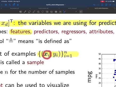
- The scalar quantity to predict is y, also called the target or label; other literature may call it the response, regressand, or dependent variable.
- The input features are represented by x, with D denoting the number of feature quantities; alternative terms include predictors and attributes.
- A dataset consists of n paired examples, each matching one feature vector with its corresponding target.
- Plotting horsepower against miles per gallon creates a scatter plot with one point for each vehicle in the roughly 400-example dataset.
- A new car with horsepower around 120 can be assigned a rough MPG prediction by inspecting nearby observations in the plot.
- Regression turns that visual intuition into a learned mapping from input features to a predicted target.
- The feature matrix X has n rows and D columns, with each row representing one vehicle and each column representing one feature.
- The feature vector for sample i is written as a row of X, while j indexes individual features.
- The target vector y stacks the n measured MPG values, and row i of X must remain paired with target y_i.
- The model predicts y with an affine linear expression: y-hat = beta_0 + beta_1 x_1 + ... + beta_D x_D.
- The coefficients beta_0 through beta_D number D+1 because beta_0 is the intercept; the residual is the difference between the true target and its prediction.
- The model describes approximate predictions, not perfect recovery of reality, and can be applied to a new vehicle whose features were not in the training data.
- A sample prediction is an inner product between the coefficient vector and a feature vector augmented with a leading 1.
- The training design matrix A is formed by adding a column of ones to X, allowing all sample predictions to be written as A times beta.
- For a new feature vector x, the prediction uses the augmented row [1, x-transpose] multiplied by the learned coefficient vector.
- Least squares chooses beta to minimize residual sum of squares, the sum of squared prediction errors across all n training samples.
- With two features, a linear model forms a plane: beta_0 sets its vertical offset, while beta_1 and beta_2 control its tilt along the two feature axes.
- Fitting the model means moving the plane to minimize the squared vertical residuals between the observed data points and their predictions.
- The Euclidean norm of a vector is the square root of the sum of its squared components.
- Residual sum of squares is the squared Euclidean norm of the difference between the observed target vector and the prediction vector.
- The general machine-learning workflow specifies a model, obtains paired training data, selects a loss such as RSS, and finds parameters that minimize it.
- For least squares, RSS varies smoothly with the coefficients and forms a bowl-shaped quadratic surface; in a one-feature example, its axes are beta_0 and beta_1.
- A contour plot shows equal-RSS ellipses, with the minimum at their center; gradient arrows point uphill and shrink toward zero near the minimum.
- The gradient stacks the partial derivatives of the loss with respect to every coefficient, and the optimum satisfies a vector equation where all those derivatives are zero.
Transcript excerpt
0:01 Okay. So today we're going to start a new unit um our first unit uh really that's on machine learning and this is about a um type [clears throat] of machine learning called regression which is basically prediction of some quantity that's like a real number or more than one real number. And um just like most of our units, we have associated with it a demo um that comes with some code that tries to solve some practical problem um using real world data. And so in this case [clears throat] we are trying to predict the fuel efficiency in miles per gallon of an automobile.
0:49 um [clears throat] from other data from what we call features uh like the number of cylinders in the engine, the horsepower in the of the engine, the weight of the vehicle and so on. So, um, the code that I'll be showing you guys, um, some screenshots of is in this demo O2 autoMPG and we're going to be using the AutoMPPG data set which we're going to uh, download from OpenML and the data is going to be in the form of a pandas dataf frame. How many of you guys have seen or heard of pandas data before? Okay, a few of you guys. Um, so
1:39 it's a really um nice it's a package within Python and it's a nice way to store and view and pre-process data. And the data frame is the main object that pandas uses. And this object has it has many data fields and it has many uh different um methods associated with it. But the three main ones are the the values um which is basically going to be the numerical values of the data set and they're going to be stored as numpy
This is the start of the transcript. Save this video free for the whole transcript, searchable and time-coded.
In this course
Related notes
Summary, takeaways, and chapters were generated by AI from the video's transcript and may contain errors. The video belongs to its creator, Prof. Schniter.