Lecture 18: Linear neural network (cont); Fully connected neural network
Overview
Burton Ma derives gradients for a layered linear network using the chain rule, showing why parameter gradients can be computed from the output layer backward. He then introduces fully connected networks with vector and matrix notation, and derives back-propagation equation BP1, including the output-layer error for least-squares loss; BP2 and BP4 are left for the next lecture.
Key takeaways
- A neuron's weight gradient follows the chain W → Z → A → C, combining the previous activation, the local activation derivative, and the downstream cost derivative.
- For a bias included as an extra weight, append 1 to the activation vector; this makes dZ/db equal to 1 and incorporates bias into ordinary matrix multiplication.
- Back-propagation avoids expanding a large network's full derivative: it computes output-layer error first, then reuses it to derive gradients layer by layer toward the input.
- In a fully connected layer with n neurons and p previous-layer neurons, including a bias unit gives a weight matrix of size n by (p + 1).
- For half squared-error loss, the gradient with respect to output activations is A − Y, so BP1 multiplies that residual element-wise by the output activation derivative.
- The 1970 Finnish master's thesis described back-propagation for interconnected functions, while Geoffrey Hinton's 1986 paper helped establish the method in neural-network research.
Chapters
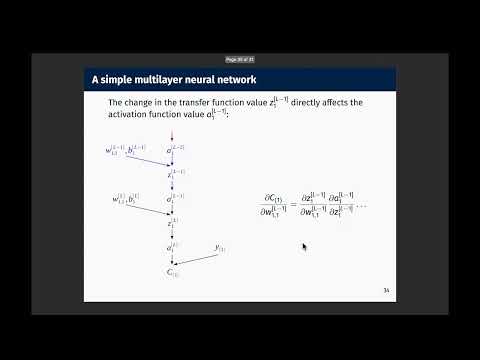
- For one training pair, changing a last-layer weight changes the cost through the sequence W → Z → A → C.
- The weight gradient combines the output error, the activation-function derivative, and the previous layer's activation.
- For m training samples, sum the individual gradients or average them by dividing by m.
- The last neuron's bias gradient follows the same chain rule as its weight gradient, but dZ/db = 1.
- The derivative of cost with respect to a previous-layer activation includes the next neuron's weight.
- That activation derivative is useful for calculating the gradients of earlier layers.
- Repeating the derivative calculation across a three-layer example yields weight and bias gradients for all three neurons.
- Gradients for earlier layers reuse cost derivatives propagated from later layers.
- Computing gradients from the last layer toward the first is the key insight behind back-propagation.
- Back-propagation applies the chain rule efficiently to networks too large for manually expanded gradients.
- Burton Ma recounts that a Finnish master's student derived the algorithm in a 1970 thesis about interconnected functions.
- A 1986 paper co-authored by Geoffrey Hinton helped popularize back-propagation for neural networks.
- The network model expands from one neuron per layer to multiple neurons, potentially with different layer sizes.
- The example has one hidden layer and one output neuron, so it maps a vector input to a scalar output.
- N superscript L denotes the number of neurons in layer L; the extra bias unit is excluded from that count.
- Each neuron receives a weight for every activation in the previous layer and an additional bias weight.
- Appending a 1 to the activation vector lets the bias be included in the same weighted sum.
- A layer's weight matrix stacks one neuron's weight vector per row, with rows equal to the layer's neuron count and columns equal to the previous layer's neuron count plus one.
- Multiplying a layer's weight matrix by the previous activation vector computes every neuron's pre-activation Z in one operation.
- Applying the layer's activation function element-wise produces its activation vector, with a trailing 1 for the next layer's bias.
- The Hadamard, or Schur, product multiplies equal-sized arrays element by element; MATLAB's dot-star operator performs this operation.
- The back-propagation notation defines δ as the gradient of cost C with respect to pre-activation Z.
- For the final layer, the chain rule gives δ as the cost gradient with respect to activation, multiplied element-wise by the activation-function derivative.
- BP1 packages the output-layer error as a vector so it can seed gradient calculations in earlier layers.
- For half the squared Euclidean error between output activations A and target labels Y, the cost gradient with respect to A is A − Y.
- The output error for this loss is therefore the element-wise product of A − Y and the output activation-function derivative.
- The lecture completes BP1 and defers BP2, BP4, and a network-training example to the next lecture.
Transcript excerpt
0:02 All right. Uh I guess we'll get started. So um just to remind you what we're doing, um we're looking at this simple linear network of neurons. Um and eventually we want to train this thing, but to train this thing we need to compute its gradient. So that's what we're trying to do here. Um at the end of the last lecture we got to uh these sets of slides. So to compute the gradient, um one way that you can do it is you can uh visualize what's happening with a picture like this. Um and so this is showing you the neuron in the last layer. Right? So here's uh the input coming from the second last layer flowing into the neuron. Neuron calculates its uh its transfer function followed by its activation function.
0:50 Um what we want is the gradient of the overall network, but if we look at the gradient of just this one neuron, what we want what we're interested in is the quantity uh if these quantities change, how does the cost change at the end? So we're looking for dW dC and dB by dC. And so the basic idea is is if you tweak W, that causes a change in Z1, which causes a change in A1, which causes a change in C. Uh and so Right? So to get the uh so the the change in W causes a change in C. So that's just your derivative dC by dW. Uh and then you just follow the path of information as it flows through the neuron. Right? So changing W causes Z to change. So that's just dZ by dW. Changing Z causes A to change. So that's
1:38 just dA by dZ. Uh and then changing A causes C to
This is the start of the transcript. Save this video free for the whole transcript, searchable and time-coded.
In this course
Related notes
Summary, takeaways, and chapters were generated by AI from the video's transcript and may contain errors. The video belongs to its creator, Burton Ma.