Lecture 17: Artifical neuron (cont); Linear neural network
Overview
Burton Ma reviews training a single artificial neuron on Fisher's Iris data, showing how MATLAB vectorization computes least-squares gradients and how learned weights define a linear decision boundary. He then builds toward backpropagation in a four-layer network, defining layer and weight notation, deriving the output-neuron gradient by the chain rule, and connecting small activation derivatives to vanishing gradients.
Key takeaways
- MATLAB can compute a single-neuron gradient across many Iris observations without explicit loops by combining matrix multiplication, elementwise Hadamard products, column sums, and averaging.
- A single neuron's zero pre-activation defines a linear classification boundary; for two inputs, its slope and intercept are determined by ratios of the learned weights and bias.
- A sigmoid neuron produces continuous scores, so binary predictions require a threshold such as 0.5; the thresholded decision boundary can remain linear.
- Backpropagation applies the chain rule along the network's information flow, multiplying the cost-to-activation, activation-to-pre-activation, and pre-activation-to-weight derivatives.
- Small derivatives of sigmoid or tanh activations can cause gradients to shrink through layers, one mechanism behind the vanishing-gradient problem.
Chapters
- The example uses Fisher's Iris data to distinguish setosa from non-setosa using sepal length and width.
- The neuron predicts a binary label: 1 for setosa and 0 for other species.
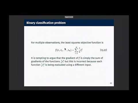
- Training minimizes a least-squares objective, requiring gradient-based optimization because the neuron includes a nonlinear activation.
- Each column of the input matrix X holds one observation, with target labels stored together in vector Y.
- Matrix multiplication computes all weighted inputs at once, and vector operations compute activations and residuals.
- A repeated residual matrix and elementwise Hadamard multiplication avoid loops; summing columns and dividing by the sample count gives the average gradient.
- The MATLAB example initializes all neuron weights to 0.5 and runs gradient descent with up to 50,000 iterations.
- The trained neuron separates setosa from non-setosa with a straight line in the two-feature plot.
- Setting the neuron's weighted input to zero gives the boundary: X2 = -(W1/W2)X1 - W3/W2, where the weights determine its slope and intercept.
- A sigmoid activation returns a real value between 0 and 1 rather than a direct binary prediction.
- A generalized Heaviside classifier with threshold 0.5 converts sigmoid outputs into class labels.
- The lecture's example reports that using sigmoid instead of Heaviside still produces a linear boundary separating the Iris classes, though the learned weights differ.
- Gradients for connected neurons follow the chain rule because each neuron's output feeds the next neuron's nonlinear function.
- The lecture moves from a single neuron to a simple four-layer network with two units per layer.
- Burton Ma adopts notation similar to Michael Nielsen's Neural Networks and Deep Learning and Grant Sanderson's 3Blue1Brown explanations.
- Layer 0 is the input layer, layer 3 is the output layer, and layers 1 and 2 are hidden layers.
- Information flows left to right through the simple feed-forward network.
- Square-bracket superscripts identify layer numbers, while unit indices distinguish neurons within each layer.
- Square units echo an input or generate a constant, while circular units compute neuron activations.
- A constant-one unit supplies the bias input, replacing the earlier practice of appending a 1 directly to the input vector.
- Each neuron combines incoming weighted activations and a bias, then applies an activation function to produce its output.
- A connection's weight is indexed sink first, then source, identifying the receiving neuron before the sending neuron.
- The sink-source ordering aligns with entries in the eventual weight matrix; reversing the indices corresponds to its transpose.
- Biases are indexed by the neuron they belong to, since the constant-one source does not need a meaningful unit identity.
- For training sample 1, the network prediction is the activation of neuron 1 in the final layer, written A₁ᴸ or Ŷ₁.
- The residual compares the target Y₁ with the network output, and the sample cost is 1/2(Y₁ - A₁ᴸ)².
- Neural-network terminology commonly calls this quantity the cost or loss function; least squares is used here for its simple derivatives.
- The output neuron's pre-activation is Z₁ᴸ = W₁₁ᴸA₁ᴸ⁻¹ + B₁ᴸ, combining its weight, previous-layer activation, and bias.
- The cost derivative with respect to a weight factors into derivatives through Z, the activation A, and the cost C.
- For least squares, the cost derivative with respect to activation is A₁ᴸ - Y₁; the activation derivative is φ′(Z), and the pre-activation derivative with respect to weight is the incoming activation.
- Small sigmoid or tanh derivatives can shrink gradients across layers, contributing to the vanishing-gradient problem and making network training difficult.
Transcript excerpt
0:01 All right, good morning everybody. Uh so this let me quickly remind you of what we were talking about in the last class. So in the last class we were looking at a single artificial neuron. Uh we computed the gradient of the neuron. Uh and then we wanted to train the neuron on a sing in a simple binary classification task. So in the binary classification task you're trying to separate two groups of data. You're trying to separate groups of data into one of two different classes. Uh and so the example we were looking at uh here was the uh iris data from um uh from Fisher's. Fisher was a statistician. Um So when you plot the iris data here you can see there's clearly two different classes, right? There's the blue and the red. We want to train a neuron so that it can
0:48 distinguish between these two um uh these two classes, right? So in other words, if we feed a neuron one of these data points, so this is like 5.5, 4.4. We feed that input into a neuron, it should spit out uh this is setosa, so it should spit out a one. Right? So the our neuron outputs a one if it's a the species of the uh sample is setosa. Or if it thinks the species is setosa, and it spits out a zero if it if it thinks the species is something else. Okay, so to train this thing uh we want to minimize the um sum of some objective function. And we chose a least squares objective function. Uh so to do that we uh it's a non-linear problem cuz the neuron is a not represents a non-linear function.
1:37 So we need some sort of um minimization algorithm, right? There's
This is the start of the transcript. Save this video free for the whole transcript, searchable and time-coded.
In this course
Related notes
Summary, takeaways, and chapters were generated by AI from the video's transcript and may contain errors. The video belongs to its creator, Burton Ma.