Lecture 16: Artifical neuron
Overview
Burton Ma explains an artificial neuron as a weighted sum of inputs, including a bias, followed by an activation function, then derives how its weights can be optimized with gradient descent. He applies the method to classify 150 Iris specimens as Iris setosa or not using sepal length and width, with MATLAB code that uses a surrogate derivative for the Heaviside activation to learn a separating line.
Key takeaways
- A neuron computes a weighted sum z = xᵀw, including a bias weight paired with an appended input of 1, then applies an activation function to produce its output.
- Sigmoid and tanh can have very small derivatives for extreme inputs, while ReLU is computed as max(0, z) and is widely used in modern neural networks.
- The Heaviside activation gives binary outputs but has zero derivative almost everywhere; the Iris example uses a surrogate derivative of 1 so gradient descent can update weights.
- For squared error ½(y − a)², a single-example gradient with the Heaviside surrogate is −(y − a)x.
- Using sepal length and width from 150 Fisher Iris specimens, one trained neuron learns a line separating Iris setosa from the other two species.
Chapters
- An artificial neuron maps an input vector to a scalar output, making each neuron a mathematical function.
- The perceptron dates to the 1950s; later progress enabled larger networks and more effective training.
- The lecture focuses on neuron structure, computing its gradient, and training one neuron for classification.
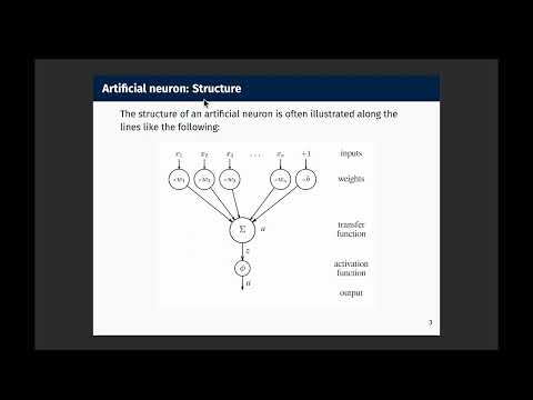
- Each input component xᵢ has a corresponding weight wᵢ that controls its influence on the neuron's output.
- Appending an input value of 1 provides a weight called the bias, which allows a nonzero response when other inputs are zero.
- The transfer function sums weighted inputs, written as a dot product such as xᵀw.
- A weighted sum alone is linear, which limits the patterns a neuron can represent.
- An activation function φ transforms the transfer value z into the neuron's final output a.
- The universal approximation theorem is introduced as a reason networks with nonlinear activations can approximate a wide range of functions.
- The sigmoid function, 1/(1 + e⁻ᶻ), maps inputs to values between 0 and 1 and can be interpreted as a probability.
- Sigmoid's derivative is φ(z)(1 − φ(z)); its small gradients at extreme inputs can hinder gradient-based learning.
- Tanh maps inputs to −1 through 1 and has derivative 1 − tanh²(z), but also saturates at extreme values.
- ReLU computes max(0, z), is simple to evaluate, and was used in the Transformer architecture described in “Attention Is All You Need.”
- The Heaviside function switches between 0 and 1, matching a binary on/off output but having zero derivative almost everywhere.
- Because a zero gradient blocks ordinary gradient descent, the lecture uses a surrogate derivative of 1 for the Heaviside function.
- An identity activation returns z unchanged and has derivative 1, making it useful for some network outputs.
- Binary classification assigns examples to one of two classes, such as cat versus not cat.
- An image can be represented as a vector by concatenating its pixel rows or columns.
- Supervised training requires labels, such as 1 for a cat and 0 for not a cat; medical-image projects may also require people to mark structures manually.
- For a labeled example, the residual is r = y − a, and the lecture uses the squared loss ½r².
- The neuron output is a = φ(z), with z = xᵀw, so the chain rule connects the loss gradient to the activation derivative and input vector.
- With the Heaviside surrogate derivative set to 1, the single-example gradient becomes −r x.
- A nonlinear activation makes the resulting objective nonlinear, so the lecture uses an iterative optimizer rather than a closed-form least-squares solution.
- For multiple examples, the method aggregates per-example residual and gradient contributions into an average squared-error objective.
- The classification task uses Ronald Fisher's Iris dataset, containing 150 specimens across three species.
- Only sepal length and sepal width are used so the examples and decision boundary can be plotted in two dimensions.
- Labels are encoded as 1 for Iris setosa and 0 for the other species; a learning rate sets the steepest-descent step size.
- The dataset is loaded with MATLAB's Statistics and Machine Learning Toolbox; the lecture notes the toolbox is needed for the built-in data.
- The measurements are arranged with specimens in rows, so the code transposes the selected sepal measurements to use column vectors.
- MATLAB string comparison identifies setosa labels, which are converted to the binary target vector Y.
- A row of ones is appended to the input matrix X so the weight vector can include the neuron's bias.
- The MATLAB implementation computes transfer values for all 150 examples with matrix multiplication, then applies the Heaviside threshold.
- Residuals are computed as Y minus the activation outputs; the code combines these residuals with X to form the batch gradient.
- The gradient is passed to steepest descent with a fixed learning rate, producing learned weights W*.
- The resulting black line separates the plotted setosa specimens from non-setosa specimens; interpretation of the specific weights is left for the next lecture.
Transcript excerpt
0:01 All right, good morning. Um, today's lecture um is about uh the neurons in an artificial network. Uh, so if you don't know how neur how a neural network works um uh I guess it's sufficient for you uh for you to know that an artificial network is made up of a bunch of neurons. uh each neuron is absurdly simple which you'll see today. Um so a neuron is just a kind of unit that computes uh some value given a vector of inputs. Uh so in other words a neuron is just a function. Uh and that's literally all it is. Um so it's inspired from biology. So the first model of an artificial neuron or an early model of the artificial neuron was somewhere in
0:48 the 50s um where someone came up with what's called the perceptron algorithm. um the neurons we use today are not much changed from then. Um so the big differences that have happened since the 50s is our ability to arrange neurons into large networks uh and to be able to train them uh effectively. Uh and so that uh I guess being able to train an artificial neuronet network was uh what won uh the Nobel Prize in physics um for uh Hinton. I can't remember the other two off the top of my head. Um uh but it's kind of a big deal uh as I'm sure you're all aware right now.
1:36 Okay. So this lecture we're going to talk about the structure of the neuron. You're going to see it's very simple. Um it basically describes a mathematical function. Um we're going to compute its gradient uh so that we can actually um optimize something uh using one of these neurons. Um so we're going to train a single
This is the start of the transcript. Save this video free for the whole transcript, searchable and time-coded.
In this course
Related notes
Summary, takeaways, and chapters were generated by AI from the video's transcript and may contain errors. The video belongs to its creator, Burton Ma.