Lecture 15: Non-linear least-squares (cont); Convexity
Overview
Burton Ma connects Gauss-Newton nonlinear least squares to multilateration: distances from known landmarks define a position-estimation problem, which he formulates with residuals and Jacobians and demonstrates in MATLAB using four landmarks and noisy measurements. He then develops multivariate convexity through chord and tangent-plane definitions, convex functions and norms, and convex sets built from half-spaces and level sets.
Key takeaways
- With exact distances, three landmarks can resolve a 2D position and four can resolve a 3D position; GPS applies the same multilateration principle using at least four satellites.
- Noisy landmark distances turn localization into a nonlinear least-squares problem: minimize the sum of squared differences between measured and position-predicted distances.
- Gauss-Newton uses the Jacobian of the residual functions to iteratively update position; in Burton Ma's MATLAB example, a starting estimate offset by 100 in both coordinates converges close to the true location with standard-deviation-1 noise.
- Convexity in multiple dimensions means that along every segment between U and V, the function value stays below the weighted average of its endpoint values.
- Positive-semidefinite quadratic forms, norms, positive sums of convex functions, and affine compositions provide common ways to construct convex objectives.
- Convex feasible regions can be built by intersecting half-spaces, and convex functions also have tangent hyperplanes that globally lower-bound their values.
Chapters
- Gauss-Newton linearizes a nonlinear least-squares objective with a first-order Taylor approximation and repeatedly solves a least-squares problem using Jacobians.
- In 2D, distance measurements to two landmarks can leave two candidate intersections; a third landmark can identify a unique position.
- In 3D, four spheres can locate a unique point under exact measurements; GPS uses distances to at least four satellites.
- The unknown parameter vector W represents the estimated position, while each known landmark position is an input to the distance model.
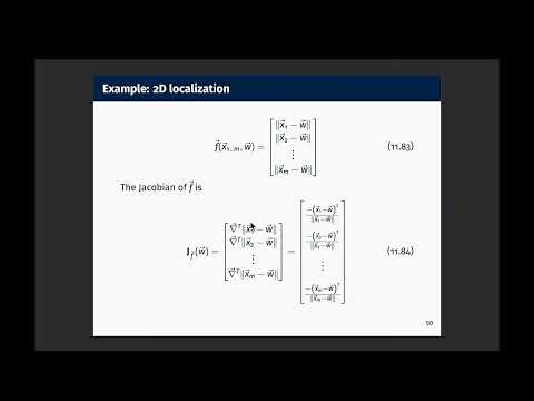
- Each residual is the measured landmark distance minus the distance predicted from W, and the objective minimizes the sum of squared residuals.
- The Jacobian is assembled from gradients of the landmark-distance functions, enabling a Gauss-Newton update.
- The MATLAB example uses four landmark coordinates and a randomly selected true 2D position, then computes each landmark-to-position distance with vecnorm.
- Normally distributed measurement noise with standard deviation 1 produces an estimate close to the true location; increasing the noise scale to 5 worsens the estimate.
- The initial estimate is deliberately offset by 100 in both coordinates, and the example shows the estimate converging near the true position.
- GPS is presented as a more sophisticated real-world application of multilateration; surveying and angle-based triangulation are also mentioned.
- A function is monotone when it is entirely non-decreasing or entirely non-increasing across its domain.
- Some optimization references describe monotonic behavior over separate intervals, but that usage differs from the whole-domain calculus definition.
- A function can decrease toward a minimum and then increase without being convex; convexity requires the graph to lie below every chord between two points.
- For scalar inputs T1 and T2, points on the connecting segment are written as (1 − θ)T1 + θT2 for 0 ≤ θ ≤ 1.
- A function is convex when its value at each point on that segment is no greater than the corresponding weighted average of endpoint values.
- For vectors U and V, the same definition applies along the segment (1 − θ)U + θV, extending convexity to multivariate functions.
- A scalar linear map AᵀW is convex because its value along a segment equals the weighted average of its endpoint values; vector-valued linear maps are built from such rows.
- Adding a constant or vector preserves convexity, making a linear map plus a translation an affine map.
- The quadratic form WᵀKW is convex when K is symmetric positive semidefinite, the multivariate analogue of a nonnegative multiple of x².
- Convexity is preserved by positive scaling, sums of convex functions, and composition with an affine map.
- A norm maps vectors in Rⁿ to nonnegative scalar lengths and satisfies zero only at the zero vector, absolute homogeneity, and the triangle inequality.
- The triangle inequality is ‖V + W‖ ≤ ‖V‖ + ‖W‖, not equality; the lecture connects this distinction to an error on Test 1.
- Examples include absolute value, the Manhattan or L1 distance, and the Euclidean or L2 distance.
- Combining the triangle inequality with homogeneity proves convexity because the segment weights θ and 1 − θ are nonnegative.
- For a differentiable convex function, the tangent line in one dimension generalizes to a tangent plane or hyperplane in multiple dimensions.
- A second-order Taylor expansion uses the gradient and Hessian; a positive-semidefinite Hessian makes the quadratic remainder nonnegative.
- Consequently, the function value at any point is at least the value of the tangent hyperplane constructed at a reference point.
- A set is convex if every segment joining two of its points stays inside the set; ellipsoids, circles, squares, and triangles are examples.
- The empty set, a singleton, all of Rⁿ, lines, and hyperplanes are also convex under the stated definitions.
- Half-spaces such as W₂ ≤ −1 and W₂ ≥ −1 are convex, and intersections of convex sets remain convex.
- Intersecting half-spaces can construct convex regions, including polygons such as the triangle formed by three linear constraints.
- A level set is defined by f(W) = c; in two dimensions it commonly appears as a level curve.
- The sub-level set f(W) ≤ c contains points on or inside the corresponding level curve, while the super-level set f(W) ≥ c contains points on or beyond it.
- Linear inequalities such as W₂ ≤ a define half-spaces as sub-level sets, and intersections of such convex sets can produce further convex regions.
Transcript excerpt
0:02 All right, good morning everybody. So, picking up where we left off from last day, we were talking about non-linear squares and we're talking about the Gauss-Newton algorithm for solving a non-linear squares problem. So, remember non-linear squares, you're trying to solve an objective function that you're trying to minimize, sorry, an objective function that looks like the sum over n values y i minus some function squared. Right, so it's a squared objective function. x i are your independent variables, your y i's are your dependent variables,
0:50 and so your non-linear model relates your observations to your model parameters w. And your independent observations via some non-linear function f. Right? Now, because this thing is non-linear it becomes difficult or impossible to find a least to find an analytic solution to this problem. So, instead what you do is you one approach that you can take is that you can linearize this thing. And when you linearize it using a Taylor series of first order Taylor series approximation you crunch through all the math, you end up with a least squares problem. Which you can now solve over and over and over again until you converge to a solution. And so, in the least squares problem
1:39 the oops, this term these terms here right, that looks like the normal equations for a regular least squares problem or for a linear least squares problem. And in fact, it is the equivalent of the normal equations. It's just now that you're using the Jacobians of the functions. Oh, sorry. Um and you can plug that solution into any uh That's the gradient. So, you can plug that's the sorry, the gradient is boom boom boom boom Uh we had an expression for the gradient somewhere. Oh, I'm sorry. That is the gradient. Let
This is the start of the transcript. Save this video free for the whole transcript, searchable and time-coded.
In this course
Related notes
Summary, takeaways, and chapters were generated by AI from the video's transcript and may contain errors. The video belongs to its creator, Burton Ma.