ISE 754 (Fall 2026) 4.4 Prod-Inv: Multiple Products
 Watch on YouTube →
Overview
Michael G. Kay compares four multi-product production-inventory formulations, showing that shared capacity with coupling constraints can remain a linear program, while exclusive resource use requires integer variables and mixed-integer optimization. He applies the models to a two-material trucking plan, explains how setup and switchover costs change schedules, and connects optimization results to weekly rolling-horizon management reports.
Key takeaways
- For multiple products sharing divisible capacity, a coupling constraint can keep the production-inventory model as a linear program when production variables are continuous and there are no setup costs.
- Exclusive use of a resource requires integer Z variables to prevent two products from using it simultaneously, so both linking-constraint formulations require mixed-integer linear programming.
- In the two-material trucking example, variable extraction costs are $120 per ton, while transport costs are modeled as setup costs of $200 per truck trip and $800 per tractor-trailer load.
- The trucking plan's optimization raises its cost from the $70,160 lower bound to $70,264 after accounting for inventory and transport decisions.
- Switchover indicator V must register a transition into production; constraints comparing current and prior Z values prevent the model from switching products without paying the associated cost.
- Rolling-horizon planning supports weekly management reports: a 26-week schedule can be re-optimized each week as demand forecasts change.
Chapters
- Each product gets its own production-inventory network, with production variables indexed by stage, period, and product.
- Coupling constraints sum product flows against shared capacity and suit continuous process production, allowing a linear program when there are no setup costs.
- Linking constraints enforce exclusive resource use through integer Z variables, making the formulation a mixed-integer linear program.
- The four formulations distinguish coupled or exclusive resources, setup costs, and switchover costs.
- The coupled model without setup costs adds one capacity constraint to the single-product model; adding setup costs introduces integer Z variables and requires mixed-integer optimization.
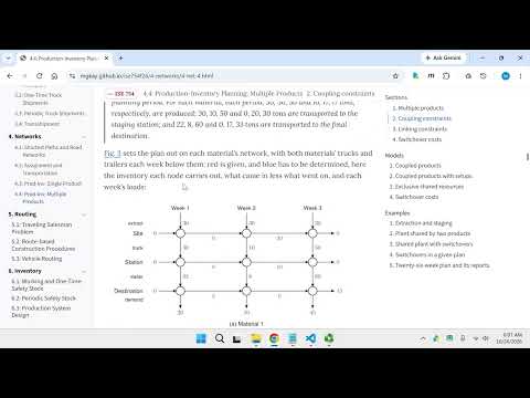
- The trucking example moves two materials from extraction to staging in trucks capped at 10 tons, then to a final destination using tractor-trailers.
- Extraction costs $120 per ton, small-truck trips cost $200, and tractor-trailer loads cost $800; each material has a 20-ton storage limit and 5 tons required at both the start and end.
- The computed lower bound is $70,160 and the optimized total is $70,264, comprising extraction, transport setup, and inventory costs.
- The full trucking problem is reduced to three periods so production, inventory, and transport flows can be calculated by hand.
- Red values represent input data; blue values are inferred primarily from flow-balance equations for both materials.
- The hand-calculated truck counts and costs match the solver's results, validating the network interpretation.
- Model 3 represents two products that share a resource exclusively; integer Z variables gate access even though they have no direct objective cost.
- Model 4 adds switchover constraints and binary V indicators, charging a cost whenever production changes from one product to another.
- A practical switchover cost can represent cleaning equipment before it can safely produce a different product.
- Z records whether a product is being made at a stage in a period, while V records whether a switchover occurs.
- The switchover constraint compares current-period Z with the previous period's Z and prevents an unpaid transition from not producing a product to producing it.
- Because the model minimizes cost, excess V indicators that would charge for unnecessary switchovers are not selected by the optimizer.
- Adding switchover costs to the example with two products changes the production profile by reducing switches and can leave a period with neither product being made.
- A 26-week production-inventory plan can generate product-specific weekly production reports, with the plan re-solved each week using updated demand forecasts.
Transcript excerpt
0:02 This is the second of two lectures on production inventory modeling as a network model. This lecture focuses on multiple products whereas the first was on a single product. This table captures the essential differences between looking at it from the point of view of a single product versus multiple products. One important distinction is what models can be solved using a linear program versus which ones require a mixed integer linear program. And that's an important difference. uh linear program essentially allows problems of any size to be solved very efficiently. Whereas mixed integer
0:51 linear programming it really is a mixed bag in terms of sometimes it can be solved uh quite easily and then other times it could be quite difficult. So whenever possible if a model is solvable as a linear program that's definitely preferable. So in the case of production inventory systems for a single product if the capacity decisions are input to the model then that could be solved as a linear program. Whereas as we saw in the previous lecture if we want the model itself to determine when to produce and when capacity was available then that needed to be modeled as a setup cost and then that required a mixed integer linear programming solution. Similarly for multiple products in the
1:39 case of what is called the joint shared resources using coupling constraints and I'll talk about that in just a minute what that means. If that's the case then it can be solved as a linear program whereas if we have exclusive resources then that's when we require mixed integer linear programming. These two figures highlight the difference between coupling constraints versus linking constraints. And coupling constraints, these are the ones that allow multiple products to be solved as a linear program. And
This is the start of the transcript. Save this video free for the whole transcript, searchable and time-coded.
Related notes
Summary, takeaways, and chapters were generated by AI from the video's transcript and may contain errors. The video belongs to its creator, Michael G. Kay.