ISE 754 (Fall 2026) 2.2 Single-Facility Minisum
 Watch on YouTube →
Overview
The single-facility minisum problem chooses a facility location that minimizes the weighted sum of transport distances, with monetary weights combining physical quantities and transport rates. A production example shows how bills of material and customer demand produce weights that place a plant in Winston-Salem, while the lecture also covers the Fermat-Weber problem, Nelder-Mead optimization, alternative location objectives, and practical distance measures.
Key takeaways
- A transport monetary weight is physical tonnage multiplied by a dollar-per-ton-mile rate, so equal physical flows can have different location importance when transport rates differ.
- With Asheville and Durham inbound weights of 40 and 10 and customer weights of 10, 20, and 30, the total weight is 110 and the weighted median places the plant in Winston-Salem.
- A facility can lose physical weight during production yet be monetary-weight-gaining: the example's outbound rate is $1 per ton-mile, compared with an inbound rate of one-third dollar per ton-mile.
- The convex Fermat-Weber minisum objective has a single global minimum, allowing centroid-initialized Nelder-Mead optimization to converge from different starting points.
- Maximin siting requires a bounded region because maximizing distance from existing facilities otherwise has no finite solution.
- A 1.14 circuity factor applied to a 121-mile great-circle distance estimates about 138 road miles, a more suitable basis for road transport cost.
Chapters
- Single-facility minisum is a cooperative location problem with a linear objective, appropriate when transport costs scale with miles, such as a truck driver paid by the mile.
- The supply chain separates into upstream assembly and downstream distribution; loads can change size between facilities, from large rail or ocean shipments to smaller delivery vans.
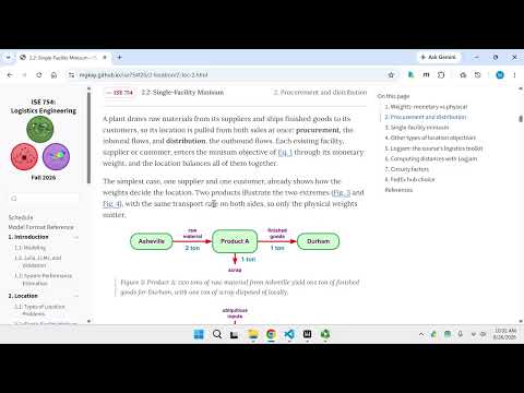
- Production must account for mass balance: 4 tons of raw material plus 1 ton of ubiquitous input yields 3 tons of finished goods and 2 tons of local scrap.
- Free on board (FOB) origin or destination specifies when ownership and transport risk transfer; these business terms generally do not change the facility location decision.
- A monetary weight, measured in dollars per mile, equals physical weight multiplied by a transport rate in dollars per ton-mile; it captures both quantity and shipping cost.
- For 60 tons of customer demand, the bill of material requires 120 tons from Asheville and 30 tons from Durham; at an inbound rate of one-third dollar per ton-mile, their monetary weights are 40 and 10.
- Outbound demand at Statesville, Raleigh, and Wilmington is 10, 20, and 30 tons, with a $1 per ton-mile rate, giving weights of 10, 20, and 30.
- The ordered weights total 110, so the one-dimensional weighted-median threshold is 55; cumulative weight first reaches it at Winston-Salem, the recommended plant location.
- For three equally weighted points, the Fermat point has 120-degree angles when all triangle angles are below 120 degrees; this is the geometric basis of the Fermat-Weber example.
- A historical Varignon frame used holes, hanging weights, and joined strings to physically find the weighted minimum-distance location.
- The optimization implementation starts at the centroid and uses the Nelder-Mead procedure to search for the minimum total cost.
- The minisum cost surface is convex, so different starting points converge to the same global minimum; Nelder-Mead probes directions and narrows its search until cost improvement falls below a stopping threshold.
- The maximin objective places a facility as far as possible from the nearest existing facilities, making it suitable for an obnoxious facility such as a garbage dump.
- A bounded region is essential: without a boundary, the maximizing location would move indefinitely far away.
- A county boundary can provide the constraint, as in searching for a Wake County site farthest from its cities and towns.
- Logjam provides tools for location analysis and supports p-norm distances: p=1 gives rectilinear distance, p=2 gives Euclidean distance, and p approaching infinity gives the maximum-coordinate distance.
- Great-circle distance is fast to calculate for many locations, but using it directly with a dollar-per-road-mile transport rate understates cost.
- A circuity factor of 1.14 converts a 121-mile great-circle distance into an estimated road distance by multiplication, avoiding the need to calculate each road route.
Transcript excerpt
0:02 We'll be talking about the single facility minisum location problem. This is a foundational problem from which we'll build out a lot of the location theory as we get into a variety of other extensions. This basic problem itself if if you remember from the previous lecture where we talked about the different types of location problems. This is an example of a cooperative location problem and it is an example of a linear objective function. In the taxonomy you had nonlinear which is essentially all of the other types of object objective functions and the minisum location problem is the single linear objective function problem that we'll be solving. Being linear makes it relatively easy to solve and also
0:53 uh it corresponds to a situation that in practice is actually appropriate in cases where for example you're paying a truck driver by the mile which is true for most cases. First concept talked about in this lecture is the difference between monetary versus physical weights. And in general, when somebody in logistics talks talks about the weight of something being transported, by default, they typically refer to the monetary weight, not the physical weight. And you'll see why that differs a lot. Even if the physical weight doesn't change, you can have differences in the monetary weight for a situation. This figure here shows the basic uh network structure. Uh this is probably
1:41 the most extensive you would think of. Here we have a single manufacturing plant and it produces a single product A. We'll call it product A. And A is composed of two major components B and C. They're both produced at two other facilities presumably at a different location. The these would be the tier one suppliers. Each unit of B is composed of a unit of
This is the start of the transcript. Save this video free for the whole transcript, searchable and time-coded.
Related notes
Summary, takeaways, and chapters were generated by AI from the video's transcript and may contain errors. The video belongs to its creator, Michael G. Kay.