ISE 754 (Fall 2026) 1.3 System Performance Estimation
 Watch on YouTube →
Overview
Michael G. Kay introduces methods for estimating production and logistics system performance, from bracketing and Little’s Law to variability-based cycle-time formulas and simulation. The lecture emphasizes that utilization must remain below 100%, explains why cycle time rises sharply near capacity, and shows how Julia discrete-event simulation can evaluate queue policies and nonstationary operations when analytical formulas are unsuitable.
Key takeaways
- For a bus route with headway H, perfect control gives average waiting of H/2 and no control gives H; taking the geometric mean of these bounds provides a practical estimate.
- Little’s Law links throughput, WIP, and cycle time, so knowing any two allows the third to be estimated for production, service, or logistics systems.
- A production resource should not be planned at 100% utilization: without spare capacity, disruptions cannot be recovered from and queues grow, while cycle time increases especially sharply above roughly 80% utilization.
- The VUT approximation attributes queueing to variability and utilization; with deterministic arrivals and processing, both SCVs are zero and the estimated cycle time is just process time.
- Repeated simulation improves estimates of stochastic performance: the FIFO example’s single-run result of 0.53 is checked against a 0.5 analytical average using 20 replications.
- Simulation supports operational details that standard analytical formulas may not handle, including shortest-processing-time priority and nonstationary schedules such as a 10-hour barber-shop day.
Chapters
- Bracketing estimates actual performance between two easier cases: perfect control as a lower bound and no control as a practical upper bound.
- For a bus headway H, perfect spacing gives an average passenger wait of H/2, while the no-control bound is H; the geometric mean of the bounds estimates actual waiting time.
- Little’s Law relates throughput, work in process (WIP), and cycle time: arrivals and departures define the system flow, and the gap between them represents items in the system.
- Manufacturing, service, and logistics systems share production-system characteristics, including demand, inputs, output, and potential scrap.
- The squared coefficient of variation (SCV) normalizes variability: deterministic timing has SCV 0, Poisson arrivals with exponential interarrival times have SCV 1, and high-variability processes can exceed 1.
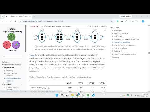
- Throughput feasibility determines the minimum number of capacity resources needed; a logistics resource could be a truck or a distribution-center loading dock, not just a manufacturing machine.
- Long-run utilization must stay below 100%, because a fully utilized system has no capacity to recover from disruptions and its queue grows without bound.
- The VUT cycle-time approximation combines variability, utilization, and process time; as utilization approaches 100%, the utilization term drives cycle time upward, making roughly 80% a common design target.
- In the pizza-delivery example, adding a fifth driver reduces estimated waiting from 20 minutes with four drivers to 12 minutes.
- Simulation is useful when analytical cycle-time approximations do not fit; the lecture presents Julia as fast enough for large-scale simulation without relying on a separate simulation package.
- A single-server FIFO simulation estimates a long-run cycle time of 0.5; one run yields 0.53, while 20 replications produce a more stable estimate near 0.5.
- Discrete-event simulation can test queue disciplines that FIFO formulas do not cover: selecting the shortest processing-time job reduces the example’s average cycle time from 0.5 to 0.29.
- Monte Carlo simulation is also used to generate Poisson arrivals and estimate system performance.
- Analytical cycle-time formulas assume stationary data; preprocessing can remove an initial demand spike, a trend, and seasonality to isolate random variation.
- A barber shop illustrates the mismatch between steady-state formulas and daily operations: it starts with no queue, and its average wait rises gradually during a 10-hour day.
- The barber-shop example takes more than 1,000 hours to reach the stationary regime assumed by the formula, so a 10-hour simulation better represents one operating day.
- Simulation can model finite or changing operating periods without requiring the system to reach long-run stationarity.
Transcript excerpt
0:10 Lecture 1.3 is the last of the three introductory lectures for the course and its topic is system performance estimation. The purpose of this lecture is to provide a common vocabulary of different techniques to model the performance of different types of systems, including logistic systems. So, it basically provides a set of characteristics of production systems, including logistic systems, that we can use when we want to develop a model. It's a technique for given a particular design of a system, be able to estimate its different
0:58 performance characteristics. The first technique for system performance estimation is sort of like estimation, sort of the sure fire technique. It's a technique called bracketing. And the idea of bracketing is that for many systems it's relatively easy to estimate the performance of the system if you assume perfect control. So, everything operates best case scenario. Nothing ever goes wrong. Everything is perfectly well operated. Turns out that you can actually characterize the performance of the system under that perfect regime. Of course, no actual system actually ever achieves
1:46 that level of perfection. At the other extreme in terms of performance, you know, systems can potentially go to infinity in terms of not performing if things break down. So, instead of the theoretical possible infinity in terms of performance, you know, going totally uh out of whack, it's more effective to look at a situation of what could be termed a practical upper bound or worst-case upper bound. And from a system's perspective, that corresponds to the case of no control. If you assume that nothing is being done to actually try to control the system so that it operates effectively, then, just like with perfect control, it turns out that there are typically
2:34 uh ways of being able to fairly effectively estimate that no control
This is the start of the transcript. Save this video free for the whole transcript, searchable and time-coded.
Related notes
Summary, takeaways, and chapters were generated by AI from the video's transcript and may contain errors. The video belongs to its creator, Michael G. Kay.