IEE 475: Lecture J3 (2026-11-10): Estimation of Abs. Perf. III (Non-Term. Sys/Steady-State Sims)
Overview
Ted Pavlic reviews confidence intervals, prediction intervals, and replication planning before applying those ideas to steady-state simulations, where initialization bias must also be controlled. For terminating systems, he shows how pilot-run variance and a desired confidence-interval half-width can estimate replication needs; for non-terminating systems, he recommends informed initialization, plotting replications to choose a warm-up period, and, after reaching 25 replications, spending remaining compute on longer runs.
Key takeaways
- For terminating simulations, estimate the replication count from a pilot standard deviation and a stakeholder-defined confidence-interval half-width; an example required 47 runs by a z approximation versus 49 by the exact t calculation.
- Confidence level and precision are different: lowering a 95% interval's confidence level narrows it by increasing the chance of missing the true mean, while adding replications narrows it without changing the nominal coverage.
- A prediction interval describes the likely range of a future output, whereas a confidence interval describes uncertainty about the mean; both can be 95% intervals but answer different questions.
- Steady-state initialization bias can be reduced by starting queues or inventories near plausible long-run levels, then using replication plots and smoothed averages to justify a discarded warm-up period.
- For steady-state runs, retain roughly 10 times as much data as the warm-up discards, build up to 25 replications, and then spend additional compute on longer runs to reduce variance and bias.
Chapters
- Lab 10 is the last assigned lab, with sequences in part one and batching, signaling, and holding in part two.
- The lab is graded out of 30 points with 50 possible, leaving room to choose how much of the two-part work to complete.
- Final presentations and reports are due Wednesday of the last class week; assigned peer reviews are due Saturday.
- Homework H covers a chi-squared analysis for a Poisson model and power analysis; homework J2 is the final assignment and can use Arena Process Analyzer to automate parameter runs.
- Simulation reports should include intervals, not just means, because each run produces a different estimate.
- Independent, identically distributed replication summaries allow standard-error estimation; observations within one run, such as adjacent customer wait times, may be correlated.
- Treating correlated within-run observations as independent creates pseudoreplication and intervals that are too narrow.
- When output is skewed, a transformation such as the logarithm may make interval methods more appropriate, but interpretation must be translated back to the original scale.
- A confidence interval represents population-mean values not rejected by the corresponding test; its half-width is the margin on either side of the sample mean.
- Across repeated experiments, a 95% procedure misses the true mean about 5% of the time, while a 99.9% interval is wider and misses less often.
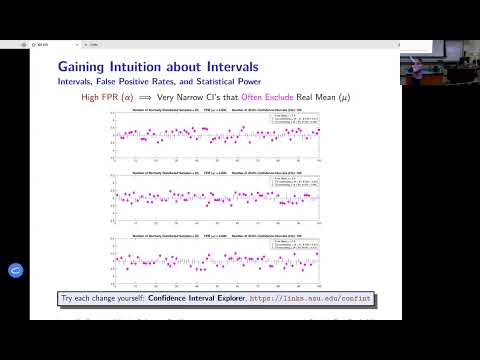
- Lowering confidence to 40% narrows intervals but makes them miss the true mean about 60% of the time.
- For a fixed data set, increasing confidence increases interval width; a 100% confidence interval spans the whole real line.
- With the confidence level fixed at 95%, increasing the sample from 20 to 200 or 2,000 observations narrows the interval while preserving the nominal error rate.
- Higher replication counts improve statistical power by reducing variability in the estimated mean.
- At the same replication count, a system with standard deviation 2.0 produces wider intervals than systems with standard deviations 1.0 or 0.5.
- The t-test statistic leads to the confidence-interval bounds by solving for population means that are not rejected by the observed sample.
- For a one-sample test, a hypothesized mean outside the 95% confidence interval is rejected at the 5% level.
- Two non-overlapping 95% confidence intervals support a conclusion that the system means differ; overlapping intervals do not establish whether a formal two-sample test is significant.
- When data are normal and there are enough observations, a 95% confidence interval can be approximated as the sample mean plus or minus twice the standard error.
- Given a confidence interval, its confidence level, and the sample count, the half-width formula can be rearranged to estimate the sample standard deviation.
- A confidence interval estimates the mean, while a prediction interval estimates where a future observation, such as the 21st data point after 20 samples, is likely to fall.
- A prediction interval is wider because it includes both population spread and uncertainty from estimating the distribution; as the sample grows, it approaches the population's central coverage range.
- For a requested quantile such as the 80th percentile, a quantile confidence interval bounds the percentile rank that contains the true quantile.
- Proportions also need uncertainty bounds: a simulation estimate of 70% should be reported with an interval rather than as an unsupported point value.
- Terminating simulations can use independent replications with different random-number seeds; Arena handles seed variation automatically.
- A stakeholder can specify a desired confidence-interval half-width, such as plus or minus one minute for average wait time, instead of specifying statistical power.
- Use the pilot estimate of standard deviation and the critical t value to solve for the required replication count; because the t value depends on the count, an exact solution requires a search.
- For roughly 20 or more replications, substituting a critical z value gives a simpler approximation, and the pilot runs already completed are subtracted from the estimated total.
- Simulation replications cost time: a call-center model may run slowly, and a Texas water-flow simulation described by Pavlic takes about 10 minutes per run.
- For the Texas wetlands study, the number of possible configurations makes exhaustive simulation impractical, so compute time and budget must shape the experiment.
- In a pilot example, 20 replications and a one-quarter-minute desired half-width gave an approximate total of 47 runs using z; the exact t-based calculation required 49.
- The Output Analyzer can calculate additional replications from a desired half-width or switch to a power-analysis approach.
- For the same five normally distributed samples, the 99% confidence interval is wider than the 95%, 85%, 10%, or 1% interval.
- A confidence interval becomes wider as its confidence level rises because it must cover the true mean more often across repeated experiments.
- Reporting a single estimate such as a 5.2-minute mean gives no uncertainty range and is equivalent to a zero-width interval.
- Non-terminating simulations aim to estimate long-run averages, such as the average demand over an indefinitely operating system.
- A finite run must choose both its total duration and the time or observation period at which measurement begins.
- Including startup transients that would not occur in the real system biases steady-state estimates.
- A common strategy is to reduce startup effects, discard a warm-up period, and calculate statistics only from the remaining observations.
- Queueing estimates from IEE 470 can provide a plausible starting queue length instead of initializing every queue at zero.
- For example, if theory predicts an average of six people in a queue at steady state, initialize the simulation near six rather than waiting for the queue to fill.
- Inventory simulations can similarly start with a realistic stock level, such as refrigerators already stocked at a Best Buy.
- Because initial-state estimates may be wrong, intelligent initialization reduces but does not necessarily eliminate the need for a warm-up period.
- Plot observations from an individual replication to identify early behavior that differs from later behavior; a cumulative average can reveal when the run begins to level out.
- A cumulative average from one run may suggest a warm-up near observation 250, but other replications are needed to check whether that pattern generalizes.
- Plotting all replications, along with moving and cumulative averages, helps reveal whether behavior settles around 250 to 300 observations.
- A half-width band across replications provides another diagnostic: visibly changing early behavior supports discarding a warm-up period rather than collecting statistics from time zero.
- As a practical transient-rejection rule, aim to retain at least 10 times as many observations as are discarded for warm-up.
- If the budget permits fewer than 25 replications, add replications up to 25.
- After reaching 25 replications, use remaining budget to extend each run, including both the warm-up and data-collection periods.
- Longer runs reduce within-replication variance and allow more transient data to be discarded, improving both precision and bias.
- Batch means offers an alternative to many separate steady-state replications: run one very long simulation and divide the post-warm-up output into batches.
- Pavlic leaves the question of how to choose batch lengths for the next lecture.
- The closing clicker question asks which quantity does not change simply by increasing the number of replications, highlighting that more replications do not automatically remove estimator bias.
Transcript excerpt
0:04 Okay. So, um looking forward here. Last lab is this week. This uh lab 10. Um remember this is a I give you a little extra time on this lab two because it's a basically a a two lab, but it's it's graded out of 30 points, but there's 50 points possible. So, there's quite a lot of um bonus here. Um it's uh you know part one covers sequences which are really helpful when building complex uh systems or patterns of of connections. Uh part two is batching signaling and holding. Signaling and holding in particular is uh is can be very helpful and very useful in building uh systems that you can sort of make interact across distances without having to build some sort of complex connection
0:53 of entities to make that happen. So, um, both of these are meant to be helpful in coming up with, uh, tools for you to use in your final project, which is why I want to make sure you saw both of them, but I also want to give you enough time to work in your final project. So, um, you know, you can kind of pick and choose these how you want to score these 30 points or if you do have the time, again, it's basically like a for another free lab. Um, then otherwise, that's the last lab. So, the rest of the lab time for the rest of the semester is basically just open labs. Uh, so we'll still have the lab times open as kind of office hours with the lab TA, but they're meant to be, you know, you can come into those times. You could spend them with the TA or you could just, you know, not having to do work on the lab
This is the start of the transcript. Save this video free for the whole transcript, searchable and time-coded.
In this course
Related notes
Summary, takeaways, and chapters were generated by AI from the video's transcript and may contain errors. The video belongs to its creator, Ted Pavlic.