IEE 475: Lecture G3 (2026-10-22): Input Modeling, Part 3 (Parameter Estimation and Goodness of Fit)
 Watch on YouTube →
Overview
Ted Pavlic explains how to estimate distribution parameters with maximum likelihood, compare candidate input models using AIC and BIC, and assess fit with plots and hypothesis tests. The lecture connects practical modeling choices to statistical cautions, including overfitting, chi-square degrees of freedom, and how sample size affects p-values.
Key takeaways
- For independent exponential observations, maximum likelihood estimates the rate as λ = 1 divided by the sample mean.
- AIC and BIC penalize extra parameters to limit overfitting; candidate models within two information-criterion units are often practically indistinguishable.
- For chi-square goodness-of-fit tests, expected bin counts should be at least five, and degrees of freedom must be reduced for parameters estimated from the data.
- A p-value measures how unusual the observed data are under the null, not the practical importance of a difference; interpret it in light of sample size and effect size.
- Increasing the significance level alpha lowers the chi-square critical value, making rejection of the null hypothesis easier.
Chapters
- Lab 8 is due Sunday; students should use the copy button in the input analyzer rather than submitting screenshots with interface controls.
- The next open lab is for gathering data for team projects, and the input modeling report should propose a system and show access to data for one or two variables.
- Every student must submit four team members by Friday so Ted Pavlic can finalize groups; the input modeling report is due the following week.
- Parameter estimation selects values such as a normal distribution's mean and standard deviation, a Weibull distribution's shape and scale, or an exponential distribution's rate.
- A location parameter shifts a distribution without changing its shape; a normal distribution has location and scale parameters.
- An exponential distribution has a rate or scale parameter but no location parameter unless a shift is added, such as a constant delay of six.
- The unbiased sample variance divides the sum of squared deviations from the sample mean by n minus 1 because estimating the mean uses one degree of freedom.
- Dividing by n instead produces a biased variance estimate when the mean is estimated from the same data.
- Equivalent variance formulas can be chosen for computational convenience, but the denominator must reflect whether the mean was estimated.
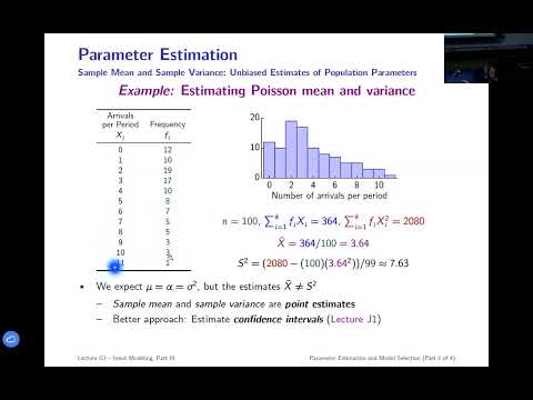
- For discrete data recorded as outcomes and frequencies, calculate the mean and variance by weighting each outcome's contribution by its count.
- A continuous-data histogram can be approximated as discrete data by treating each bin midpoint as an outcome and its bin count as the frequency.
- In the Poisson example, the estimated mean is 3.64 and the estimated variance is 7.63, even though a Poisson distribution has one parameter that determines both.
- Probability asks about outcomes when parameters are known; likelihood evaluates candidate parameters after the observed data are fixed.
- For independent observations, the joint likelihood is the product of the individual probability densities, with each observation sharing the same unknown parameter.
- Maximizing the exponential likelihood gives the rate estimate λ = 1 divided by the sample mean, providing a mathematical justification for the familiar estimate.
- An MLE can be derived by differentiating the joint likelihood with respect to a parameter, setting the derivative to zero, and solving.
- The Poisson MLE is the sample mean, even though the sample variance also estimates the population variance; parameters do not generally equal every corresponding sample statistic.
- Computers maximize log-likelihood because taking the logarithm converts products into sums and avoids numerical underflow from multiplying many small densities.
- A Weibull or gamma distribution can include the exponential as a special case when its shape parameter equals one, so the extra flexibility cannot reduce maximum likelihood.
- An empirical distribution with 13 parameters can match one week's histogram perfectly, yet generalize poorly to a different week's data.
- A simpler two-parameter gamma fit may be less exact on the training histogram but more useful on future observations because it is less prone to overfitting.
- AIC balances fit against model complexity using the log-likelihood and number of parameters; lower AIC is preferred.
- BIC also penalizes extra parameters, with a penalty that grows with sample size, and is useful when one candidate is known to be the true data-generating model.
- Models within two AIC or BIC units of the best model are difficult to distinguish; a difference greater than four provides stronger evidence against the higher-scoring alternative.
- For 100 observations generated from an exponential distribution with mean five, AIC ranks Weibull first, while exponential, gamma, and Weibull all fall within two AIC units.
- BIC selects the exponential in the example because its stronger complexity penalty favors the true one-parameter model.
- The input analyzer ranks models by AIC by default and flags close alternatives; fitted Weibull or gamma shape parameters near one indicate an effectively exponential fit.
- Ted Pavlic advises against Arena's input analyzer because its square-error ranking selects a lognormal model for this example, which he considers an inappropriate fit.
- Choosing the best candidate family does not guarantee an adequate fit; a goodness-of-fit test checks whether the observed data are consistent with the fitted distribution.
- The null hypothesis is that the data came from the fitted family and parameters; the alternative is that they did not.
- A Type I error rejects a true null hypothesis, while a Type II error fails to reject a false null hypothesis.
- Setting alpha to zero means never rejecting the null, while alpha equal to one means always rejecting it; lower alpha requires a larger chi-square critical value.
- A p-value is the probability, assuming the null hypothesis, of observing data at least as far from the null as the results obtained.
- One coin flip landing heads provides little evidence about fairness; 900 heads in 2,000 flips can produce a very small p-value even if the practical bias is modest.
- Large samples can make tests detect negligible differences, while small samples can produce uninformatively high p-values.
- Reporting an effect size alongside statistical significance helps stakeholders judge whether a detected difference matters in practice.
- In a two-tailed binomial test, a 6-to-1 result across seven games has a p-value of 12.5%, so it does not meet an alpha level of 0.05.
- Seven wins out of seven would meet the example's 5% threshold, while a close 4-to-3 series offers little evidence that one team is better.
- Statistical power, equal to one minus beta, helps determine how many games or observations are needed to detect a specified difference.
- The same low-power problem can affect close elections; runoffs and additional data can help distinguish near-tied outcomes.
- The chi-square goodness-of-fit test compares observed counts in bins with expected counts under the proposed distribution.
- For a fitted distribution, the expected count in a bin is the sample size multiplied by the model's probability of falling in that bin.
- Expected counts should be at least five; combine adjacent bins when necessary, including for skewed distributions such as the exponential.
- Degrees of freedom account for the number of bins and the parameters estimated from the data, which changes the chi-square critical value.
- The lecture closes with a short-answer attendance question asking whether increasing Type I error alpha raises or lowers the chi-square critical value.
- The preceding rule gives the answer: increasing alpha makes rejection easier, so the critical value decreases.
Transcript excerpt
0:08 Okay. So, good morning. Uh lab schedule um lab 8's due this Sunday. [clears throat] TA uh emailed me this morning to let me know that they're not able to come to class today, but will be available uh during the lab at their their um their link, their Zoom link. So, look at the announcement for that or go to the office hours web page, instructor web page to find that. Um, but otherwise, today's lab is not a lab that you need the arena input analyzer because we're using our own input analyzer. So, um, that shouldn't be necessary to have access to the lab computers. Um, the lab will still be open. So, I guess if you wanted to have access to the lab computers, you could do that. Um, but, uh, so that's the idea there. Again, that's due Sunday. When
0:55 you do that input analyzer uh exercise, try not to use screenshots. I mean, every one of those uh images, those graphs you come out of there has a copy button above it. You hit copy and you can paste it right into there. So already I'm getting uh I'm getting lab reports that have the buttons across the top that say how to export the image in the screenshot. And so um so try to avoid you know like responsible try to do responsible screen cap and so you know if there's another way to get it that's actually maybe even quicker like that's the better way to go and that's going to look like a better uh image for your report. So make use of that. Um otherwise next week is not lab 9. It's an open lab that allows you to collect
1:44 data or work with the data for your team. So, it's a lot like doing uh lab
This is the start of the transcript. Save this video free for the whole transcript, searchable and time-coded.
Related notes
Summary, takeaways, and chapters were generated by AI from the video's transcript and may contain errors. The video belongs to its creator, Ted Pavlic.