IEE 475: Lecture G2 (2026-10-20): Input Modeling, Part 2 (Selection of Model Structure)

Overview

Ted Pavlic explains how to select input-model structure before fitting probability distributions, using Arena examples to show how bimodal and repeated-peak metal-detector times can reveal distinct populations or feedback loops. He then covers histogram binning, choosing among Arena distribution families, converting Poisson arrival counts into exponential interarrival rates, avoiding overfitting, and using QQ plots before PP plots to assess model fit. The lecture also prepares students for Lab 8 and the project input-modeling report, including team formation and data-source planning.

Key takeaways

A bimodal metal-detector passage-time distribution can be represented as a mixture of short unflagged passages and longer flagged passages, rather than forced into one unimodal input distribution.
Repeated histogram peaks separated by roughly 60 seconds can indicate feedback in the system, such as flagged people being checked and sent through screening again; validate that structural hypothesis by observing the real process.
Use sample CDFs to inspect distribution shape without choosing histogram bins: repeated values create jumps for discrete data, while flat regions and steep segments can expose gaps and modes.
When arrivals are approximately constant-rate, estimate the rate from fixed-window counts: divide the fitted Poisson mean by the observation-window length, then use the resulting rate for exponential interarrivals in Arena.
Prefer the simplest distribution consistent with system knowledge; automated tools may select flexible gamma models that fit historical data better but generalize worse than an exponential or Erlang.
Assess distribution families with QQ plots before PP plots: QQ plots reveal tail and shape mismatches, while PP plots help compare central fit after suitable parameters have been fitted.

Chapters

0:00 Lab 8, Project Reports, and Team Formation

Lab 8 uses supplied data to practice fitting input models, preparing students for the final project's first technical deliverable.
The new custom input analyzer accepts pasted columns or spreadsheets and exports graphics as PNG or SVG; Ted Pavlic recommends exporting figures instead of using screenshots.
Each student must submit four proposed teammates, including themselves, by Friday; a shared editable spreadsheet and course discussion spaces help students find groups.
The input-modeling report is due the following week and doubles as a project proposal, describing the system, data source, and models fitted to pilot data.

8:24 Why Input Distributions Matter in Simulation Models

In a queueing model, changing interarrival-time or service-time distributions can change output even when the distributions have identical means.
Supply-chain simulations depend on demand and lead-time distributions, while reliability models depend on failure-time behavior.
Testing whether data fit a proposed distribution is important, but identifying a sensible distribution family in the first place is the harder task.

10:24 The Metal Detector Example and a Misleading Exponential Fit

The Arena baseline represents people as entities, a metal detector as a capacity-one resource, passage as a seize-delay-release process, and departures as a dispose block.
Given only a 30-second mean and standard deviation, an exponential distribution seems plausible because it has equal mean and standard deviation.
The exponential model allows passage times approaching three minutes, which conflicts with the physical scale of walking through the detector and signals that summary statistics alone are insufficient.

13:31 Explaining Bimodal Passage Times with a Mixture Model

The observed passage-time histogram is bimodal, so fitting one familiar unimodal distribution would hide meaningful system structure.
Splitting observations at 50 seconds produces a short-time group resembling an exponential with mean about 4 seconds and a longer group resembling a normal distribution with mean about 70 seconds and standard deviation about 5 seconds.
Of 1,000 observations, 588 fall in the short-time group and 412 in the long-time group, suggesting a mixture with probabilities of roughly 59% and 41%.
The sample CDF reveals the same modes through steep accumulation regions separated by flatter regions, without requiring a histogram bin-width choice.

18:20 Representing Security Outcomes in Arena and Testing Scenarios

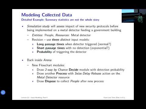
The mixture becomes an Arena flowchart with a two-way chance Decide block and separate process blocks for short, unflagged passage and longer, flagged passage.
The probability of triggering the detector is a model parameter that can be calibrated to observed data or changed for scenario analysis.
At a 10% detection probability, the example mixture has a mean passage time of 11 seconds; at 90%, the mean rises to about 60 seconds.
The likely population matters operationally: trained employees may need less security staffing than occasional visitors unfamiliar with screening procedures.

23:44 Repeated Histogram Peaks Suggest Screening Feedback

A second passage-time example has auxiliary peaks spaced about 60 seconds apart, with fewer observations in each successive peak.
One plausible explanation is that flagged people undergo a checking process and return through the detector, adding roughly 60 seconds per repeat.
The repeated groups have similar widths, supporting a shared screening-time process plus an accumulating time offset.
The hypothesis should be checked by observing the real system; repeated peaks alone suggest, but do not prove, repeated screening.

31:29 Revise the Flowchart Before Fitting a Complicated Distribution

The feedback model sends every person through the detector, routes flagged people through a check, and loops them back for another screening attempt.
Each loop adds detector time and approximately 60 seconds of checking, producing the observed sequence of peaks.
The example loop is intentionally simplified and may not represent a real security operation, which could prioritize checked people or limit repeat screenings.
A call center illustrates the same principle: a simple arrivals-service-departures overview can require a much more elaborate internal flowchart to explain its observed times.

34:17 Choosing Histogram Bins Without Mistaking Shape

Histograms and sample CDFs should be examined rather than relying only on summary statistics; continuous-data histograms are especially sensitive to bin width.
A square-root-of-sample-size heuristic gives an initial bin count, such as 100 bins for 10,000 observations, but it is only a starting point.
Too many bins produce sparse counts that obscure shape, while too few bins make distinct patterns look nearly uniform.
For discrete data, use one bin per possible outcome; combining outcomes can create bins centered on values that are not part of the distribution's support.

40:38 Arena Distribution Families and Physical Intuition

Arena's available building blocks include beta, continuous, discrete, Erlang, exponential, gamma, Johnson, lognormal, normal, Poisson, and triangular distributions.
Choose a family using physical knowledge as well as shape: ask whether data are discrete, bounded, memoryless, additive, or correlated with other processes.
The goal is a useful model for future operational analysis, not a perfect reproduction of historical observations.
Core distributions such as exponential, normal, uniform, beta, triangular, gamma, and Weibull are preferred starting points when their assumptions fit.

45:07 Distinguishing Discrete from Continuous Data

Narrow, tall histogram spikes separated by gaps can indicate a discrete variable with only a few repeated outcomes.
A sample CDF is built from sorted observations and their ranks; repeated discrete values form vertical jumps, while continuous observations produce a smoother progression.
Arena's Disc function can encode a user-specified discrete probability mass function through its cumulative probabilities.
The Cont empirical distribution is a last resort for continuous inputs because copying historical observations directly may generalize poorly to future conditions.

49:53 Normal, Exponential, Weibull, and Erlang Selection Rules

A normal distribution is a reasonable default when only an unbounded or virtually unbounded mean and standard deviation are known, and it also suits symmetric additive processes.
For nonnegative data with a known mean and little else, an exponential is a natural candidate; its mean equals its standard deviation and its memorylessness corresponds to a constant rate.
Weibull generalizes the exponential with a shape parameter that allows failure rates to vary over time; shape equal to one recovers the exponential.
Erlang distributions are physically interpretable as sums of exponential stages and provide another way to represent positive durations.

53:44 Convert Poisson Arrival Counts into Exponential Rates

For a Poisson count over an interval of length tau, the mean count alpha equals the underlying arrival rate lambda multiplied by tau.
Counting arrivals in fixed windows can be easier than recording every interarrival time; estimate lambda by dividing the fitted Poisson mean by the window length.
In the example, about 49.9 arrivals per 10-minute interval implies roughly 4.99 arrivals per minute, which can parameterize an exponential interarrival model in Arena.
The conversion is appropriate when the arrival process can reasonably be treated as having a constant rate.

58:31 Prefer Parsimonious Models to Automated Overfitting

Flexible families such as gamma may rank highly because their extra parameters fit historical data more closely, even when a simpler family better reflects the system.
If a fitted gamma shape is near one, compare it with an exponential; if it resembles an Erlang, ask whether the extra flexibility is justified.
The updated custom analyzer penalizes additional parameters, unlike the older Arena Input Analyzer's squared-error ranking, which could favor overly flexible models.
Students should justify selecting a more complex distribution when a simpler family appears to fit comparably well.

1:02:02 Use QQ Plots First, Then PP Plots to Validate Fit

A QQ plot compares sorted observations with quantiles from a hypothesized distribution; a roughly straight-line relationship supports the family, using the fat-pencil test as a visual check.
Systematic QQ-plot departures can guide model changes: excess observations in both tails suggest a heavier-tailed family, while curvature can reveal skew.
A PP plot compares empirical and hypothetical cumulative probabilities and is useful for distinguishing fit in the middle after the tails have been assessed.
The recommended workflow is to inspect the QQ plot, fit parameters, then use the PP plot as a final visual validation alongside statistical tests such as chi-square or Kolmogorov-Smirnov.

Summary, takeaways, and chapters were generated by AI from the video's transcript and may contain errors. The video belongs to its creator, Ted Pavlic.