ENEE 684 Lecture 18 | Ring Resonators and Optical Frequency Combs
 Watch on YouTube →
Overview
Ergun Simsek explains how ring-resonator geometry, dispersion, coupling, and loss determine optical frequency-comb behavior, then demonstrates a numerical workflow from mode solving to comb prediction. He connects free spectral range, quality factor, finesse, and photon lifetime to practical design limits, and uses FDFD, FEM, and the Lugiato-Lefever equation to model a silicon nitride resonator producing a comb with roughly 250 nm bandwidth.
Key takeaways
- Use group index rather than effective index when calculating ring-resonator FSR; for a 10 μm-radius silicon example with group index 4.2, the FSR is about 9.1 nm.
- Loaded Q is governed by both intrinsic and coupling losses through 1/QL = 1/Qi + 1/Qc, and the smaller component Q dominates the result.
- For the lecture’s example resonator, QL of about 15,500 implies a photon lifetime near 12.8 ps, roughly 2,470 optical cycles or 14.5 ring round trips.
- Integrated dispersion can be computed by sampling effective index across wavelength, fitting the data, and extracting FSR and coefficients such as D2 and D3 for LLE simulations.
- A combined mode-solving, dispersion-analysis, and LLE workflow predicts a roughly 250 nm-wide comb from the example silicon nitride ring pumped at 1.06 μm.
Chapters
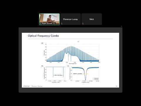
- A continuous-wave laser pumps a ring coupled to a bus waveguide, and nonlinear processes generate comb lines.
- A 1550 nm pump can produce a broad comb, potentially spanning an octave with lines near 1f, 2f, and 3f.
- The lecture’s workflow runs from mode solving and integrated dispersion to Lugiato-Lefever equation simulations of output power.
- Free spectral range is the spacing between adjacent resonances; in frequency it depends on group index and ring length, with ring length equal to 2πr.
- Use group index, not effective index, to calculate FSR; detector bandwidth must exceed the frequency spacing to resolve comb lines.
- Resonator linewidth is measured at the half-maximum level, while intrinsic loss includes material and bending loss and coupling loss comes from energy transfer between the bus and ring.
- Loaded quality factor follows 1/QL = 1/Qi + 1/Qc, so the smaller of Qi and Qc largely determines QL.
- For a silicon ring with radius 10 μm, effective index 2.4, group index 4.2, and a 1550 nm operating wavelength, the circumference is about 62.8 μm and the approximate mode number is 97.
- The example gives an FSR of about 9.1 nm and a 0.1 nm linewidth, producing a finesse near 91 and a loaded Q near 15,500.
- A propagation loss of 3 dB/cm corresponds to an intrinsic Q on the order of 10⁵, much higher than the loaded Q, indicating that coupling dominates.
- The loaded photon lifetime is about 12.8 ps for the example resonator.
- At a 1550 nm pump, the optical period is about 5.17 fs; dividing the roughly 12.8 ps photon lifetime by the period gives about 2,470 cycles, matching QL/(2π).
- The ring’s round-trip time is about 0.88 ps, so the photon lifetime spans roughly 14.5 round trips, matching finesse divided by 2π.
- A 12.5 GHz linewidth-based bandwidth provides a practical check against photodetector and modulation bandwidth requirements.
- At 10 Gbit/s, a 100 ps bit period is longer than the example lifetime; faster modulation can be limited by resonator photon storage.
- Simsek compares transmission spectra for κ² values of 0.05 and 0.015, showing that weaker coupling produces narrower, sharper resonances.
- Coupling is set by the gap and dimensions of the bus waveguide and ring, including their widths and heights.
- Critical, under-, or over-coupling may be selected according to the resonator’s intended operation rather than simply maximizing transferred pump power.
- The numerical model treats the ring, substrate, and cladding as homogeneous material regions and uses cylindrical coordinates.
- Because the structure is symmetric along z, the mode profiles can be represented on a two-dimensional r-z cross-section with an angular propagation factor.
- The solver’s purpose is to obtain resonant modes and effective indices needed for later dispersion and comb calculations.
- A resonant field must return to its starting phase after a round trip, giving the approximate condition βr·rc = m for integer azimuthal mode number m.
- Taking the curl of Maxwell’s curl equations yields the electric-field wave equation used as the starting point for numerical solvers.
- Simsek emphasizes that spatial changes in permittivity matter: generally, ∇·(εE) = 0 does not imply ∇·E = 0.
- The FDFD derivation retains the permittivity-gradient terms that arise at material interfaces, unlike the simplified assumption ∇·E = 0.
- The angular dependence is represented by an exponential with integer m, reducing angular derivatives to multiplication by −jm.
- Finite differences discretize the r and z derivatives for the three electric-field and three magnetic-field components.
- Eliminating selected angular field components produces coupled equations in r and z for the remaining field profiles.
- The coupled equations contain both β and β², making the original eigenvalue problem second order in propagation constant.
- Introducing an auxiliary field f = βa converts the system into a first-order eigenproblem.
- The conversion doubles the matrix size but returns the propagation constant and field profiles through a standard eigenvalue solve.
- For a silicon nitride ring with a 23 μm central radius, 1.5 μm width, and 0.7 μm height, Simsek shows electric and magnetic field profiles and an effective index near 1.79 for one mode.
- The FDFD solver is available in MATLAB and Python and can calculate effective indices for complex ring geometries.
- A rectangular-grid torus example produces profiles resembling Bessel functions, although material boundaries introduce field discontinuities.
- The rectangular-grid FDFD implementation is first-order accurate, while the FEM approach is introduced as a higher-accuracy alternative.
- The FEM solver uses the curl-curl electric-field equation and triangular meshes to represent the ring cross-section.
- The mesh distinguishes high-index and low-index regions, such as silicon nitride and silicon dioxide.
- FEM basis functions enforce continuity of tangential electric fields and accommodate jumps in normal components across material interfaces.
- FEM converts the differential equation into integral equations by testing it with basis functions and integrating over the domain.
- Integration by parts reduces second derivatives to first derivatives and yields a generalized matrix eigenproblem.
- The stiffness matrix contains curl operations, while the mass matrix contains field-overlap integrals.
- Boundary conditions and appropriate basis functions are essential to represent the field behavior at material boundaries.
- The FEM eigenproblem can take integer mode number m as input and solve for wavelength, or use a specified wavelength to estimate m.
- A noninteger estimated m is an approximation consequence of representing propagation across the ring with a single radius.
- FEM convergence is shown to improve at second order, and effective indices sampled across wavelengths provide data for integrated dispersion.
- Integrated dispersion is formed from resonance frequencies relative to the pump mode and the FSR, with coefficients such as D2 and D3 describing departures from uniform spacing.
- The MATLAB example uses a silicon nitride ring with 23 μm central radius, 890 nm width, 670 nm height, and a 1.06 μm excitation wavelength.
- The mode solver reports an effective index of about 1.85 and approximately 89% modal overlap within the waveguide.
- A second script samples effective index from 750 nm to 1.5 μm in 10 nm steps, fits a fourth-order polynomial, and extracts FSR, D2, D3, and resonance wavelengths.
- The resulting integrated-dispersion data is passed directly to the LLE simulation workflow.
- The LLE search varies normalized pump power f and detuning α; a single stable soliton appears in the example at f = 1.44 and α = 2.1.
- With a quality factor of 1 million, the simulated output shows regularly spaced comb lines and about 250 nm of bandwidth around a 1.06 μm pump.
- Simsek says MATLAB and Python versions of the solvers are available, though he reports MATLAB solving one spectral-integrate problem in 3.5 seconds versus about 30 seconds in Python.
- The assignment is to choose a ring radius from 40 to 200 μm, select materials and pump wavelength, estimate FSR, run mode and LLE solvers, and submit a labeled comb-spectrum figure.
Transcript excerpt
0:14 All right. Uh today we will talk about ring resonators and optical frequency combs. I think let's see. Okay, that's good. extra small. All right. Okay. Like here we have a bus wave guide. It is like there's like a laser CW laser continuous wave laser excited at 1550. So the light propagates through the wave light. Then some of the energy gets transferred to the rimator. And thanks to those that non processes when you collect the light from the other end of the bus wave guide and then you take the
1:02 FL transform of it you get this optical frequency come okay again like input is 1550 get the output it's a uh a com today we were just discussing you can use smaller rings and you can make uh like octave uh white like octave like 1 f 2 f you know 3f right so you you can write really uh wide um uh bandwidth of frequenc generation. So today first like we will throw so many equations okay so many equations about these frequenc generators then we will try to understand what those
1:51 numbers mean then we will use our uh FM finite element method based mode solver to obtain the first integrated dispersion spectrum then this com line okay com spectrum output power. So in the in like two lectures before uh Ronak was here and he showed us how we can use Lle equation to obtain the output spectrum. So that solver requires parameters such as D2 like second coefficient of integrated dispersion. Um so we will see how we can obtain them numerically. Okay. All right. Again there will be so many equations. For example, one of them is
2:40 like free spectral range. So free spectral range if you have a spectrum uh
This is the start of the transcript. Save this video free for the whole transcript, searchable and time-coded.
In this course
Related notes
Summary, takeaways, and chapters were generated by AI from the video's transcript and may contain errors. The video belongs to its creator, Ergun Simsek.