ENEE 684 Chapter 5: Geometrical Optics (Part 2)

Overview

Ergun Simsek develops geometrical-optics design methods using ABCD ray-transfer matrices, showing how to calculate ray propagation, form images, and choose lens spacing for beam expanders. He connects the matrix conditions B = 0 and C = 0 to imaging and collimated beam expansion, then discusses practical lens trade-offs—aberration, numerical aperture, coatings, and chromatic correction—and introduces laser-resonator stability and a confocal-microscopy design assignment.

Key takeaways

For an imaging system, B = 0 in the total ABCD matrix makes output ray height independent of launch angle, so rays from one object point converge to the same image point.
For an afocal beam expander, C = 0 keeps collimated input rays collimated; |A| gives the beam-diameter expansion ratio.
A Galilean expander with focal lengths -5 cm and +25 cm needs 20 cm lens spacing and expands a 2 mm beam to 10 mm without the intermediate focus of a Keplerian layout.
High numerical aperture and low f-number make tight focusing possible but increase aberration sensitivity; the lecture gives f/2 as a threshold below which lens-form choices such as plano-convex deserve particular attention.
Achromatic doublets use converging and diverging elements to bring separated wavelengths closer to a shared focus, making them useful for broadband illumination and fluorescence microscopy.
Ray tracing can identify practical best focus by minimizing RMS ray deviation over candidate axial positions, rather than assuming a real lens has one perfect focal point.

Chapters

0:00 ABCD Matrix Conventions and the Small-Angle Approximation

Geometrical optics tracks ray height and propagation angle rather than wavelength, phase, or polarization.
Free-space propagation over distance d uses the matrix [[1, d], [0, 1]]; a dielectric slab of thickness L uses L/n in the propagation term.
A thin lens of focal length f has a lower-left matrix term of -1/f; use centimeters for distances and radians for angles.
Curved-interface ray matrices reduce to Snell's law in the flat-surface limit, with the small-angle approximation sin θ ≈ θ.

3:00 Composing Optical Systems in Ray-Path Order

A multi-element system is represented by multiplying the matrices for each lens and propagation segment.
Because matrix multiplication is not commutative, the first element encountered by the ray appears at the far right of the product.
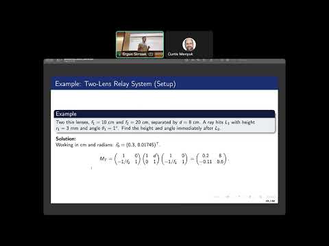
The example system contains two converging lenses with focal lengths 10 cm and 20 cm, separated by 8 cm.

6:00 Calculating Ray Height and Angle Through Two Lenses

The example ray enters the first lens 3 mm off-axis at 1°; the inputs are converted to 0.3 cm and approximately 0.01745 radians.
Multiplying the two lens matrices and the 8 cm propagation matrix gives the overall transfer matrix.
The calculated output is about 2 mm in height and 1.29° in angle; the free-space matrix determinant is checked to equal 1.
Once the optical elements are fixed, the system matrix can be reused for different input rays and detector locations.

10:00 Why Imaging Systems Require the ABCD Matrix B Term to Vanish

The output height is r₂ = A r₁ + B θ₁, so rays leaving one object point at different angles generally arrive at different heights.
Setting B = 0 makes r₂ independent of the input angle, bringing rays from the same object point to a common image point.
When imaging is achieved, A gives the signed transverse magnification: its magnitude sets image size and its sign indicates orientation.
Lens spacing can be treated as a design variable and selected to make the system's B term zero.

13:00 Deriving the Thin-Lens Equation with Ray-Transfer Matrices

The object-to-image system is modeled as propagation by d₁, a thin lens of focal length f, and propagation by d₂.
Setting the composite matrix's B term to zero yields d₁ + d₂ = d₁d₂/f.
Rearranging gives the Gaussian thin-lens equation, 1/f = 1/d₁ + 1/d₂.
The magnitude of the image magnification is d₂/d₁; the sign convention identifies whether the image is inverted.

17:00 Applying the Imaging Condition to a Two-Lens System

For the earlier two-lens layout, the object-to-first-lens propagation matrix is added to the existing lens-gap system matrix.
A 4 mm-high object is placed 30 cm before the first lens; the output propagation distance is chosen by setting the full system's B term to zero.
The worked result is approximately 5.1 cm beyond the second lens, with an inverted image about 1.48 mm high.
In free space the determinant should be 1; across media with different refractive indices, the relevant determinant ratio is n₁/n₂.

22:00 Choosing Lens Forms for Focusing and Beam Expansion

Plano-convex, biconvex, and positive-meniscus lenses are converging; biconcave and plano-concave lenses are diverging.
In the ABCD lens matrix, converging lenses use positive f and diverging lenses use negative f, regardless of the exact surface shape.
Meniscus lenses are commonly selected to reduce aberrations, while Fresnel lenses use stepped surfaces to provide optical power in a thinner form.
Lens selection should account for the source, wavelength range, optical power, aperture, and application rather than price alone.

30:00 Spherical Aberration, Best Focus, and Lens Aperture

A spherical lens sends marginal rays and near-axis rays to different focal locations, producing spherical aberration and preventing a perfect single-lens focus.
A best-focus location can be estimated by tracing rays over candidate z positions and choosing the position with minimum RMS deviation.
The f-number is focal length divided by aperture width; numerical aperture describes the focusing cone and is important when tightly focusing on small targets.
High-NA, low-f-number systems tend to show stronger aberrations; Simsek recommends considering plano-convex lenses for simple, narrow-bandwidth setups, especially below about f/2.

36:00 Aspheric Lenses and Chromatic Aberration Correction

Aspheric surfaces depart from a sphere to reduce aberrations; Simsek notes they can cost roughly five times as much as a regular lens.
Refractive index varies with wavelength, so blue and red light can focus at different locations in an ordinary lens.
Achromatic doublets combine a converging and a diverging element, often using different glasses, to bring two wavelengths to nearly the same focus.
The C and F spectral lines used as examples are approximately 656 nm (red) and 486 nm (blue); achromats are useful in broadband and fluorescence microscopy.

42:00 Fraunhofer Lines and Comparing Lens Aberrations

Fraunhofer absorption lines are dark features in the solar spectrum; the lecture connects them to wavelength-specific absorption by atoms and molecules.
MATLAB ray-tracing code is offered to compare a BK7 biconvex singlet with a cemented converging-diverging lens combination.
The illustrated doublet substantially reduces the spread in focal positions compared with the single lens.
For a single laser and narrow bandwidth, a simple plano-convex lens may suffice; multiple wavelengths or broadband sources favor an achromatic doublet.

48:00 Lens Coatings, Fresnel Thickness, and Beam-Expansion Uses

Anti-reflection coatings matter especially in high-power systems; verify the coating's performance at the operating wavelength, such as 780 nm.
For ultrafast laser applications, thick optical elements can be undesirable; Fresnel designs can replace a roughly 2 cm-thick lens with one around 5 mm thick.
Beam expansion can reduce intensity on a sensitive detector such as an avalanche photodiode or enlarge a 1 mm beam to illuminate a 10 mm sample.
The two basic beam-expander layouts are Keplerian, using two positive lenses, and Galilean, using a negative lens followed by a positive lens.

54:00 Keplerian and Galilean Beam-Expander Design Conditions

A Keplerian expander focuses the input beam between its two positive lenses, which can raise intensity and risk damage or ionization in high-energy applications.
The lens separation for a collimated afocal expander is set by the signed focal-length sum: f₁ + f₂.
A Galilean design can be shorter because one focal length is negative; for f₁ = -5 cm and f₂ = 25 cm, the separation is 20 cm.
For parallel input rays to remain parallel, the overall matrix must have C = 0; beam expansion additionally requires |A| > 1.

1:00:00 Worked Galilean Expander: Fivefold Beam Enlargement

The example uses a -5 cm diverging lens and a +25 cm converging lens with a collimated 2 mm-diameter input beam.
The ABCD matrix condition C = 0 gives a required lens separation of 20 cm, equal to -5 cm + 25 cm.
The resulting magnification is 5, producing an output beam diameter of 10 mm.
Commercial expanders may add meniscus elements and other lenses to reduce edge aberrations beyond the basic two-lens design.

1:06:00 Laser Resonators and the Stability Problem

A laser uses an energized gain medium and a cavity with a highly reflecting mirror and a partially transmitting mirror to build up and extract light.
Resonator geometries include parallel-plate, confocal, concentric, and combinations of curved mirrors with separations related to their focal lengths.
A stable cavity must keep rays circulating between mirrors rather than drifting beyond the resonator boundaries.
ABCD matrices will be used to derive stability limits and guide mirror spacing and curvature; the detailed condition is deferred to the next lecture.

1:11:00 Confocal Fluorescence Microscopy Design Assignment

The assignment asks students to research fluorescence confocal microscopy and explain its purpose, operation, and basic optical layout.
The design scenario uses a 532 nm green excitation laser and a sample emitting at 582 nm, with components selected from Thorlabs.
Students must justify choices such as beam expansion, dichroic filters, lens numerical aperture, and other optical parts.
A possible $5,000 budget makes component trade-offs part of the design; students may consult AI for checking or targeted help but should not copy generated answers.

Summary, takeaways, and chapters were generated by AI from the video's transcript and may contain errors. The video belongs to its creator, Ergun Simsek.