EE 330 Lecture 2026 10 22 Ch6 BJT#3

Overview

The lecture develops practical methods for analyzing BJT circuits: assume an operating mode, write current and voltage relations, solve efficiently with loop equations or a Thevenin equivalent, then verify that the assumed mode is physically consistent. Examples cover NPN and PNP biasing, saturation, two-stage amplifiers, complementary power stages, characteristic curves, breakdown, and temperature effects; the closing review also distinguishes the active-mode relations from the approximate 0.2 V saturation model.

Key takeaways

For an unknown BJT operating region, assume active mode, solve using VBE ≈ 0.7 V and IC = beta × IB, then verify the resulting collector-emitter voltage; an impossible node voltage means the transistor is not in active mode.
A single loop can simplify base-current calculations: with an emitter resistor RE and base resistor RB, IB = (V supply - 0.7) / [RB + (beta + 1)RE] under the active-mode model.
A BJT base divider is loaded by base current; replacing it with a Thevenin source, such as 5 V and 33.3 kΩ for the 15 V, 50 kΩ/100 kΩ example, makes that loading explicit.
Two-stage BJT bias cannot generally be solved as two independent circuits because Q2 base current changes Q1's collector branch; an isolated first pass should be followed by recalculation.
SPICE automates the simultaneous circuit equations, but hand-derived current paths and operating-region checks are still needed to design circuits and recognize implausible simulation results.
Electrical breakdown can sharply increase BJT current, but sustained heating, rather than the voltage event alone, is what commonly causes permanent junction damage.

Chapters

0:00 BJT Lecture Plan and Midterm Logistics

The lecture continues Chapter 6 BJT examples and adds temperature effects and other device characteristics.
The second midterm is scheduled for the following Thursday, with a Tuesday review covering MOSFETs and BJTs.
Students are reminded to bring ID and use both available submission attempts to improve their result.

1:45 Solve an NPN Circuit by Assuming Active Mode

For an NPN transistor with beta = 100, a 5 V base supply through 100 kΩ, a 10 V collector supply through 2 kΩ, and a grounded emitter, first test the active-mode assumption.
Using VBE = 0.7 V gives IB = (5 - 0.7) / 100 kΩ = 0.043 mA, then IC = beta × IB = 4.3 mA.
The collector voltage is 10 V - (2 kΩ)(4.3 mA) = 1.4 V, which exceeds the approximate 0.3 V active-mode boundary used in the lecture.
The resulting emitter current is IE = IC + IB = 4.343 mA; the active-mode assumption is consistent.

8:34 Set Up PNP Analysis with Signed Terminal Voltages

For PNP circuits, label voltages as VEB and VEC rather than using the NPN-oriented VBE and VCE convention.
The example cannot be in cutoff: zero current would leave about 5 V across the emitter-base junction.
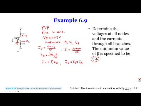
Under an active-mode assumption, VEB = 0.7 V, but the unknown terminal voltages prevent directly calculating the branch currents.
Use IC = beta × IB and IE = IC + IB together with resistor and junction-voltage equations to reduce the unknowns.

16:00 Use a Single Loop to Find Base Current

A loop from the 5 V supply through the 1 kΩ emitter resistor, the 0.7 V junction, and the 10 kΩ base resistor avoids solving a large simultaneous system.
Substitute IE = (beta + 1)IB into the loop, giving IB = (5 - 0.7) / [10 kΩ + (beta + 1)(1 kΩ)].
With beta = 30, the denominator is 41 kΩ and IB is about 0.105 mA; IE is about 3.25 mA.
The factor (beta + 1) multiplying the emitter resistance reflects that emitter current is about (beta + 1) times base current.

22:34 Reject the Active Assumption and Analyze Saturation

The calculated active-mode collector voltage is outside the circuit's physically possible supply range, so the active-mode result must be rejected.
In saturation, use the approximate VEC = 0.2 V model and do not apply the active-mode equation IC = beta × IB.
Write the resistor-loop equations and IE = IC + IB, then solve for the branch currents and node voltages.
After solving, compare the forced current gain IC / IB with beta = 30; a value below beta is consistent with saturation.

33:53 Why BJT Voltage-Divider Bias Needs Care

A common DC-bias circuit uses two resistors to set the base voltage and an emitter resistor to establish current.
Unlike a MOSFET gate, a BJT base draws current, so the base voltage is not automatically the unloaded voltage-divider result.
The voltage-divider approximation is reasonable only when base current is small compared with divider current.
Thevenin reduction makes the divider's loading effect easier to include in the BJT calculation.

36:33 Replace the Base Divider with Its Thevenin Equivalent

For a 15 V divider with 50 kΩ and 100 kΩ resistors, the open-circuit Thevenin voltage is 15 × 50 / (50 + 100) = 5 V.
With the voltage source shorted, the resistors are in parallel, giving RTH = 50 kΩ || 100 kΩ ≈ 33.3 kΩ.
The reduced circuit places a 5 V source in series with 33.3 kΩ at the BJT base.
This equivalent accounts for base-current loading without repeatedly analyzing the original divider.

40:20 Calculate and Verify the Divider-Biased BJT

Assuming active mode, calculate base current from the 5 V Thevenin source and 0.7 V base-emitter drop.
Reflect the emitter resistance to the base side: the effective denominator includes RTH + (beta + 1)RE, not simply RTH + RE.
Use IB to calculate IC and IE, then determine the collector and emitter voltages.
Check that the resulting collector-emitter voltage remains above the lecture's approximate 0.3 V active-mode threshold; otherwise redo the analysis in saturation.

44:37 Why Two-Stage BJT Bias Requires Iteration

In a two-stage amplifier, the collector of Q1 drives the base network of Q2, so the stages load one another.
Current in a resistor connected to Q1's collector is not necessarily equal to IC1 because some current can feed Q2's base.
A first pass can isolate the stages to estimate voltages and currents, but the second stage's base current changes the first-stage result.
Recalculate the coupled currents and voltages in a later pass to improve the initial approximation.

48:09 Approximate Two-Stage Bias with Beta Approaching Infinity

The simplified first pass treats beta as infinite, making base currents approximately zero and allowing voltage-divider calculations.
For Q1, a 5 V base estimate and VBE = 0.7 V give IE1 ≈ (5 - 0.7) / 3 kΩ.
Approximate IC1 as IE1, then use the 15 V supply and Q1's 5 kΩ collector resistor to estimate VC1.
Use the interstage voltage, a 0.7 V junction drop, and Q2's 2 kΩ emitter resistor to estimate IE2, then verify both transistors' operating regions.

53:33 Exact Multistage Equations and the Role of SPICE

An exact two-stage solution requires simultaneous loop equations, resistor-current relations, and transistor relations such as IC1 = beta × IB1 and IE1 = IC1 + IB1.
Interstage current conservation must include Q2's base current; for example, a branch current can split into Q1 collector current and IB2.
The full circuit can produce roughly 16 equations and 16 unknowns, which can be solved with matrix methods.
SPICE solves circuit equations behind the scenes, but understanding the equations remains necessary for circuit design and interpreting or correcting simulation results.

59:19 Complementary BJT Stages for Power Amplification

A complementary stage pairs an NPN and a PNP transistor, with the input applied to their bases and the output driving a load.
The arrangement is introduced as a power-amplifier structure relevant to class A, B, and C amplifier studies.
Unlike a small-signal example, the output can drive loads such as a speaker or solenoid.
Changing the input and supply conditions changes which transistor conducts, so analyze each operating case separately.

1:00:21 Test Transistor On and Off Assumptions Against Circuit Voltages

For complementary circuits, start with a proposed on/off state and check whether the implied base-emitter voltage and current direction agree with the supplies.
A conducting junction requires roughly 0.7 V of forward bias; an assumed current path that requires current to flow against the available voltage is inconsistent.
The lecture tests cases with a 5 V input and then a modified negative supply, using node polarities to rule out impossible states.
Checking both-transistors-off assumptions is also useful: zero current fixes node voltages, which may create an impossible 5 V base-emitter difference.

1:10:01 Common-Base and Common-Emitter Curves, Including Breakdown

In common-base operation, the base is grounded and collector current is compared with emitter current; in active mode their ratio is approximately alpha.
In saturation, collector current is much smaller relative to emitter current than in the active region.
Common-emitter curves relate collector current to base current and show saturation at low VCE, followed by the active region.
Excessive VCE can trigger electrical breakdown and a sharp current increase; sustained current generates heat that may damage or destroy the junction.

1:13:53 Temperature, Scaling, and BJT Operating-Mode Review

The lecture states that BJT beta tends to increase with temperature, relating the change to increased carrier mobility.
BJT devices can be scaled by reducing junction dimensions, although the geometry is less intuitive than MOSFET channel width and length.
The closing review summarizes cutoff, active, and saturation operation, including the active relation IC = beta × IB and the approximate 0.7 V base-emitter drop.
The lecture contrasts the active-mode voltage check with the approximate 0.2 V saturation voltage and reminds students of the Tuesday MOSFET and BJT review.

Transcript excerpt

0:01 Okay. We're going to get started. So, in last lecture we went through a couple of examples on BJT and demonstrate how different problems can be different can be solved through different angles. And also you can see how the proper problems can be formulated. So, today we're going to go over a few more examples and we're going to discuss just a few minor things about BJT like a temperature effect and so on. So, we're going to go through those. Uh just a reminder our second midterm is next Thursday. So, it's a a week from now. And on Tuesday we'll do a review session

0:49 which is going to cover both MOSFETs and BJTs. Um there's a few more um like exam oriented examples and stuff like that. So, hopefully you guys will do better than the first uh midterm. Um yeah, other than that I'll send a reminder as well what you need to do. So, for the midterm it's the same thing you guys go through that library and uh with your ID ready. Uh yeah, you stay in the exam room. You know, you have you you you you have two chances to do all the problems and then you know, make sure you you do both uh uh chances before you um yeah, you can submit twice. Just make sure that you get the best out of the two

1:36 uh two chances you have, okay? Any questions? You have any more? Okay, very good. So, um here let's look at the another example and we've got a couple today and maybe three or four more before we conclude this chapter. Um the reason we're looking at different examples is really looking at how this problem problems can be formulated in a different ways. Like looking at um given

This is the start of the transcript. Save this video free for the whole transcript, searchable and time-coded.

Related notes

Summary, takeaways, and chapters were generated by AI from the video's transcript and may contain errors. The video belongs to its creator, Wireless Power Transfer.