Dynamics (MIT 16.07) - Lecture 3: State Space, Numerical Integration, Energy, and Lyapunov Stability
Overview
Prof. Zac Manchester introduces state-space modeling and numerical simulation, showing how to express the pendulum as a first-order system for MATLAB ode45 or Python solve_ivp. He demonstrates that forward Euler can inject energy and become unstable even with small time steps, then uses pendulum energy to establish motion bounds, explain Lyapunov stability, and preview deriving equations of motion from energy.
Key takeaways
- State-space form turns the pendulum’s second-order equation into ẋ = [θ̇, −(g/L) sin θ] for x = [θ, θ̇], the format required by standard ODE solvers.
- Forward Euler injects energy into an undamped pendulum, with a positive leading error proportional to Δt²; making the time step smaller delays instability but does not eliminate it.
- MATLAB ode45 automatically adapts step size and is suitable for routine simulation, but long-term numerical energy drift still requires checking against physical invariants.
- The pendulum’s conserved energy, ½mL²θ̇² + mgL(1 − cos θ), gives explicit bounds on both angular speed and angle, confining motion to a region in state space.
- A positive, radially unbounded Lyapunov function with V̇ ≤ 0 establishes stability, while strict decrease away from equilibrium establishes asymptotic stability.
- Energy differentiation recovers the single pendulum equation without force diagrams, but one conservation equation cannot determine the dynamics of a system with multiple degrees of freedom.
Chapters
- The previous lecture compared minimal pendulum coordinates, using one angle, with Cartesian x and y coordinates plus a length constraint.
- Numerical integration of constrained coordinates caused constraint drift; Baumgarte stabilization adds feedback to reduce constraint error.
- MATLAB is the course standard for hardware labs because its toolboxes and drivers are more reliable across operating systems; Python is acceptable for homework simulations.
- The lecture reviews state-space form and numerical integration before developing kinetic and potential energy.
- Lyapunov stability connects energy-like functions to bounded motion and control.
- The closing preview uses pendulum energy to derive dynamics, leading toward Lagrangian methods.
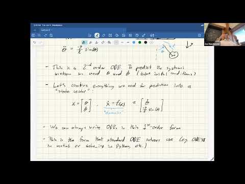
- With angle measured from vertical, the pendulum equation is θ̈ = −(g/L) sin θ.
- The state x = [θ, θ̇] contains the initial angle and angular velocity needed to predict future motion.
- The equivalent first-order dynamics are ẋ = [θ̇, −(g/L) sin θ]; any higher-order ODE can be converted by stacking variables into a state vector.
- Numerical solvers accept this form, including MATLAB ode45 and SciPy solve_ivp.
- Many engineering ODEs are nonlinear and lack practical analytic solutions, so numerical methods are central to simulation.
- An initial-value simulation requires a first-order state equation and initial state.
- MATLAB ode45 and SciPy solve_ivp both use Runge-Kutta 4(5) methods by default, with results affected by tolerance settings.
- Explicit, forward, or Euler integration advances the state using xₖ₊₁ = xₖ + Δt f(xₖ).
- Each step approximates the solution curve with a short straight segment along its current tangent.
- Smaller Δt can reduce local approximation error, but the pendulum example shows that small steps alone do not guarantee stable long-term behavior.
- The demonstration initializes the pendulum at θ = π/4 and uses MATLAB ode45 to produce the expected oscillation.
- ode45 adjusts its step size automatically to control estimated error, rather than requiring a fixed Δt.
- Forward Euler at 100 Hz adds energy and makes the oscillation grow; increasing the rate to 1,000 Hz delays the blow-up but does not eliminate it.
- Over long simulations, ode45 also exhibits numerical energy loss, visible as a shrinking trajectory in the θ versus θ̇ state plot.
- Discretization can alter physical properties such as stability and conservation, even when the continuous equations are correct.
- Zac Manchester advises against using explicit Euler for these simulations because its pendulum energy error grows over time.
- Check conservative systems for energy or momentum drift, constrained systems for constraint violations, and damped systems for decreasing energy.
- Numerical damping or energy growth should be treated as simulation error unless the physical model includes those effects.
- Particle kinetic energy is T = ½mv², while near-Earth gravitational potential energy is U = mgz.
- For a 1 kg particle falling 1 m from rest, the lost potential energy becomes kinetic energy, giving speed magnitude √(2g).
- A linear spring stores U = ½kx², where k is stiffness and x is displacement from equilibrium.
- For two point masses, gravitational potential is U = −Gm₁m₂/r; the same external gravitational field applies to spherical bodies.
- Forces derived from a position-dependent potential satisfy F = −∇U; differentiating ½kx² gives the spring force −kx.
- Conservative forces exchange kinetic and potential energy without changing total energy E = T + U.
- Friction, drag, and damping are non-conservative examples because they remove mechanical energy and depend on velocity.
- The lecture distinguishes drag, which often scales with speed squared, from linear damping, which scales with speed.
- For a pendulum of length L, kinetic energy is T = ½mL²θ̇².
- Measuring height from the lowest position gives gravitational potential U = mgL(1 − cos θ).
- Differentiating total energy and substituting θ̈ = −(g/L) sin θ makes the kinetic and potential energy rates cancel.
- The resulting Ė = 0 confirms energy conservation for the undamped pendulum.
- The initial energy E₀ stays constant, so the kinetic term gives an upper bound on angular speed: |θ̇| ≤ √(2E₀/(mL²)).
- Setting kinetic energy to zero at a turning point gives an angular bound from cos θ = 1 − E₀/(mgL).
- Together, the angle and angular-velocity bounds define a box in the θ, θ̇ state space that the trajectory cannot leave.
- A numerical ode45 trajectory stays within the energy-derived bounds despite small integration error.
- A system is Lyapunov stable around an equilibrium if trajectories starting nearby remain within a bounded region around it.
- A Lyapunov function V(x) is positive away from the equilibrium, zero at the equilibrium, and radially unbounded when it grows without bound as the state grows.
- If V̇ = (∂V/∂x)f(x) ≤ 0, trajectories cannot climb to higher V levels, giving stability.
- For the undamped pendulum, conserved energy supplies an energy-like function whose constant level sets bound motion.
- If V̇ is strictly negative away from equilibrium, the system is asymptotically stable: trajectories tend toward the equilibrium over time.
- An undamped pendulum can remain on a periodic orbit because its energy is constant, so it is stable without being asymptotically stable.
- For a controlled system ẋ = f(x,u), choosing u to make V̇ negative can produce a provably stabilizing controller, even when V is not physical energy.
- When Lyapunov conditions hold only in a region, that region can define a basin of attraction rather than global stability.
- In discrete time, energy change is measured by ΔEₖ = Eₖ₊₁ − Eₖ rather than by the continuous-time derivative Ė.
- Substituting the forward Euler pendulum update yields a leading energy-error term proportional to Δt²g² sin² θₖ.
- That term is nonnegative and generally positive, so Euler systematically adds energy to the undamped pendulum.
- Reducing Δt slows the energy growth but cannot remove the instability for any nonzero step size.
- Starting from E = ½mL²θ̇² + mgL(1 − cos θ), differentiation gives Ė = mL²θ̇θ̈ + mgL sin θ θ̇.
- Setting Ė = 0 and dividing by the common factors yields θ̈ + (g/L) sin θ = 0, matching the force-based pendulum equation.
- This shortcut avoids a free-body diagram and coordinate transformations for this conservative, single-degree-of-freedom example.
- Energy conservation alone gives too few equations for a multi-degree-of-freedom system such as a double pendulum, motivating more general Lagrangian methods.
Transcript excerpt
0:01 So, let's see. Last time, last time we sort of did our uh kind of finished up our Newtonian review stuff. Uh we talked a whole bunch about coordinates and reference frames and all that good stuff. Hopefully that's enough to get us started and I think the rest will just kind of intermix as we go as we need it. Um, so it's not that fun. So I don't want to like just inundate you with more of that than we have to. So I think that's enough to be dangerous and then we can fill in the fill in the gaps as we go. And then we did the pendulum, right? Uh, a couple different ways. We
0:48 saw the sort of what what I would call, you know, minimal coordinates, right? uh with the just the single angle versus like a what I might call a maximal coordinates or cartisian uh situation where we had explicit xy coordinates plus a constraint and we simulated that and saw there's some weird things that can happen when you try to simulate that with an OD integrator uh namely right we got this like weird constraint drift behavior where the length was wiggling around and changing and that messed up our dynamics and then we talked a little bit about this idea called boundar stabilization where you stick a PD controller in the uh in the dynamics when you simulate so that you can sort of make sure that constraint is satisfied even when you've got numerical errors and stuff like that. So that's a rough summary of last time. Any questions about any of that stuff from last time? Okay. Uh okay. So this time oh I want to mention too I got a a a
1:39 feedback thing about mat lab versus
This is the start of the transcript. Save this video free for the whole transcript, searchable and time-coded.
In this course
Related notes
Summary, takeaways, and chapters were generated by AI from the video's transcript and may contain errors. The video belongs to its creator, MIT Robotic Exploration Lab.