2NM4 Week 6 - Optimization
Overview
Optimization is framed as minimizing an objective subject to constraints, with method choice driven by available derivative information, function smoothness, dimensionality, and evaluation cost. The lecture compares bracketed methods such as golden-section search and Brent's method with open methods including Powell, Nelder-Mead, gradient descent, Newton and trust-region methods, then derives equality-constraint approaches and nonlinear least squares via Gauss-Newton and Levenberg-Marquardt.
Key takeaways
- Golden-section search contracts a unimodal bracket by about 0.618 per iteration without derivatives; Brent's method can accelerate convergence with interpolation while retaining golden-section fallback steps.
- Nelder-Mead can optimize a black-box function without gradients by moving a simplex through reflection, expansion, contraction, and shrink operations, but may need many evaluations.
- Newton optimization can solve an exact quadratic in one iteration, but its dense Hessian linear solve may cost O(n^3), making the method impractical for very large parameter spaces.
- A penalty weight that is too small permits constraint violations, while an excessively large weight worsens conditioning; Lagrange multipliers instead introduce constraints as equations in a coupled system.
- Gauss-Newton approximates the least-squares Hessian with residual-Jacobian information and works best when residuals are small; Levenberg-Marquardt adds damping to blend this local method with gradient descent.
- Stochastic gradient descent reduces per-update computation by sampling subsets or directions in high-dimensional parameter spaces, which is one reason it is useful for training neural networks.
Chapters
- Optimization seeks an input vector x that minimizes an objective, often representing cost, subject to equality and inequality constraints.
- Maximization can be rewritten as minimization of the negative objective.
- Iterative methods depend on initial guesses and basins of attraction; global-convergence strategies aim to reach a useful basin but are not guaranteed.
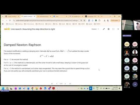
- Line search assumes a proposed direction is correct and chooses how far to move along it.
- A damping factor alpha scales the Newton step: alpha = 1 gives the full step, alpha below 1 reduces overshoot risk, and alpha above 1 can accelerate progress but may overshoot.
- Small damping improves caution at the cost of slower convergence, much like adjusting a neural network learning rate.
- A line search can fit a quadratic using the current function value, gradient, and trial function value, then choose the fitted minimum as the next step.
- Backtracking evaluates successively shorter steps to find one that improves the objective.
- These strategies spend additional function evaluations, so practical solvers trade robustness against computational expense.
- A trust-region method tracks a radius around the current point where a local quadratic model is considered credible.
- Unlike line search, which trusts the direction and adjusts distance, a trust region limits the step and can reconsider the direction.
- Solvers shrink or expand the region according to how well the actual function change matches the local model; update rules are implementation-specific.
- Nonconvex objectives can contain multiple local minima, so a local optimizer may settle in a basin that is not globally best.
- Periodic objectives and the two-variable Egg Holder function illustrate rugged landscapes with competing minima.
- Global-search approaches include multistart optimization, genetic algorithms, simulated annealing, particle swarm, and watershed methods.
- An inequality constraint can prevent an objective from decreasing indefinitely and make the constrained optimum lie on the feasible boundary.
- The lecture illustrates why finding a boundary optimum can be harder than minimizing an unconstrained function.
- In multiple dimensions, defining useful brackets is difficult, motivating open methods for many practical problems.
- A bounded minimization method evaluates points around a candidate minimum and fits a parabola through three function values.
- The parabola's minimum supplies a new trial point, and comparisons with existing values determine how to update the bracket.
- Keeping both possible bracket contractions balanced makes the method behave consistently across branches.
- Golden-section search chooses interior points so either bracket update retains the same short-to-long interval ratio.
- That self-similar ratio yields a constant interval contraction of about 0.618 per iteration.
- The method uses function values rather than derivatives and is dependable for unimodal objectives, but converges linearly.
- A log-error plot for golden-section search is approximately linear, illustrating its first-order convergence.
- The candidate minimum can move back and forth within the bracket while the interval itself steadily contracts.
- The fixed contraction makes golden-section search predictable, though it can require many evaluations.
- Inverse quadratic interpolation uses several function-value samples to predict a minimum more aggressively than golden-section search.
- The faster proposal can fail when the objective is not locally quadratic, so a bracket remains important.
- Brent's method combines interpolation with golden-section steps, using the safer bracket update when interpolation is unsuitable.
- Brent's method can fall back to golden-section steps near sharp corners such as those created by an absolute-value term.
- On irregular objectives, the fallback preserves progress even when a quadratic interpolation proposal is poor.
- The method is generally faster than golden-section search when interpolation works, while retaining a bracket-based safety mechanism.
- Open methods are useful in multiple dimensions, where practical bracketing is usually difficult.
- Gradient-free methods require only objective evaluations; gradient-based methods use first derivatives, and Newton methods also use second derivatives.
- Derivative availability, objective smoothness, and the cost of each function evaluation determine which method is practical.
- A black-box objective maps an input vector x to a scalar value, such as cost or a model score.
- Multi-objective goals, such as improving a course mark while reducing study time, are often combined into a single scalar objective.
- Powell's method and Nelder-Mead can optimize without requiring analytic gradients.
- Powell's method starts from a point and searches along supplied directions, often coordinate axes such as x and y.
- It performs sequential one-dimensional minimizations and uses displacement between resulting minima to construct new directions.
- For locally quadratic functions, the constructed directions can be conjugate, reducing the zigzag associated with steepest descent.
- Initial directions in Powell's method can be arbitrary; later directions are derived from the sequence of line-search minima.
- The method can follow a narrow valley, as illustrated with the Rosenbrock banana-shaped objective.
- Repeated minimizations increase evaluation cost; the example required about 19 iterations, and expensive function calls can dominate runtime.
- Nelder-Mead, also called the downhill simplex or amoeba method, uses a simplex: an interval in 1D, triangle in 2D, and tetrahedron in 3D.
- It ranks simplex vertices by objective value, then reflects, expands, contracts, or shrinks the simplex to explore lower values.
- The method uses function evaluations rather than derivatives and stops as the simplex's size or hypervolume becomes small.
- The Rosenbrock and Himmelblau examples show a simplex moving through difficult landscapes toward low objective values.
- The illustrated Nelder-Mead run takes roughly 80 iterations, compared with about 19 for the Powell example, but is presented as a robust black-box option.
- The method retains previously evaluated vertices to limit extra work during each reflection, expansion, or contraction.
- Steepest descent moves opposite the objective gradient, with a step size that acts as a damping coefficient or learning rate.
- Gradient descent can zigzag in narrow valleys because successive steepest directions may undo earlier progress.
- Stochastic gradient descent samples subsets or directions of a large parameter space, reducing work per update; it is used to train neural networks.
- For a scalar objective, the gradient is a vector and the Hessian is the matrix of second derivatives.
- Newton optimization solves a linear system involving the Hessian and gradient to update the parameter vector.
- Newton's method converges in one iteration on an exact quadratic from any valid starting point, but a dense Hessian solve can cost O(n^3).
- A zero gradient identifies a stationary point, which may be a minimum, maximum, or saddle point rather than a minimum.
- Nelder-Mead seeks low function values and generally will not find a saddle point; Newton methods can target stationary points through the gradient equation.
- Trust-region Newton methods limit the local quadratic assumption, shrinking the region after poor predictions and expanding it after successful steps.
- An equality constraint such as x² + y² = 1 can be written as a residual g(x) = x² + y² - 1 = 0.
- A penalty method adds a weighted constraint violation, such as a multiple of |g(x)| or g(x)², to the objective.
- A penalty that is too small fails to enforce feasibility; an excessively large penalty can make the system poorly conditioned.
- The Lagrangian combines the objective with equality constraints weighted by multiplier variables.
- Taking derivatives with respect to the multipliers recovers the equality constraints, while derivatives with respect to x give stationarity conditions.
- The method treats multipliers as additional unknowns and turns equality-constrained optimization into a coupled unconstrained root-finding problem.
- The resulting Newton system combines the objective Hessian, constraint Jacobian, its transpose, and a zero block.
- This block-structured system is typically indefinite, so standard positive-definite solvers such as conjugate gradient may not apply.
- The lecture points to block methods and the Schur complement as useful tools for solving constrained systems.
- A parameterized model f(x; β) is compared with observed values, producing one residual for each data point.
- The least-squares objective is the sum of squared residuals, rᵀr, minimized over the parameters β.
- Fitting many parameters from fewer observations is underdetermined; matching data points to parameters instead becomes a root-finding problem and risks fitting noise.
- The residual Jacobian J contains derivatives of residuals with respect to model parameters.
- Gauss-Newton approximates the Hessian of the sum-of-squares objective with a matrix based on JᵀJ, omitting terms multiplied by residuals.
- That approximation is most useful near a fit, where residuals are small, and yields an update that can be computed with robust linear-algebra methods.
- Levenberg-Marquardt adds a tunable multiple of the identity matrix to the Gauss-Newton system.
- When the tuning parameter is large, the update behaves more like gradient descent; nearer the solution, it approaches Gauss-Newton's faster local updates.
- The lecture identifies Levenberg-Marquardt as a common nonlinear curve-fitting method and relates neural-network training to optimizing a large parameter set.
Transcript excerpt
0:00 Optimization. Optimization is fun. Optimization is useful. Uh, loading. Loading. Loading. Slideshow. Run. Good thing about optimization is you guys already know how to do it. Um, optimization has been a part of your life literally since you started breathing. To be frank. What we're going to do is we're going to try and like define some of the steps. Generally speaking, you want to find some value x subject that minimizes some function, right? Typically, this would be the objective function. Whatever you're trying to minimize, usually it's cost, right? The typical one is that you you want to minimize the amount of money that you have to pay or moreover you
0:47 want to get the most that you can for the same amount of money, right? So, you want to minimize some objective subject to some constraint. So, um, uh, I don't know, you need to spend $15 at this store to make your mom happy, and you don't want to spend so much money, but you also need at least, you know, more than a positive number of bananas or something like that, right? So, you're going to minimize an objective. You're going to have an equality constraint, something that has to equal a total number. And then you're typically you're going to have an inequality constraint. This guy is hard. telling you right now not covered in this course. This guy we will if independent research projects somebody wants to go into interior point methods all of that funny business for
1:35 general optimization by all means that would be really cool. Um yeah G is the list of equality constraints. Notice all these are vectors right? You have a vector argument you have a vector of functions equality constraints that you all need to solve. vector of inequalities. Um, if
This is the start of the transcript. Save this video free for the whole transcript, searchable and time-coded.
In this course
Related notes
Summary, takeaways, and chapters were generated by AI from the video's transcript and may contain errors. The video belongs to its creator, Numerical Methods for Engineering.