Stanford AA203 Optimal and Learning-Based Control | Spring 2026 | Lecture 2: Optimization Theory

Overview

This lecture from Stanford Online's AA203 Optimal and Learning-Based Control course delves into classical optimization theory, focusing on necessary and sufficient conditions for optimality in unconstrained and constrained problems. It introduces gradient methods for iterative optimization, discusses the properties of convex functions, and explains the Lagrange multiplier theorem for equality-constrained optimization, laying the groundwork for advanced control topics.

Key takeaways

For unconstrained optimization, a local minimum x* requires ∇f(x*) = 0 (necessary) and H(x*) positive semi-definite (necessary). If H(x*) is positive definite, x* is a strict local minimum (sufficient).
Convex functions simplify optimization: any local minimum is global, and ∇f(x*) = 0 is both necessary and sufficient for global optimality.
Gradient descent iteratively updates x_{k+1} = x_k - α * ∇f(x_k), aiming to decrease f(x) at each step.
The choice of descent direction (e.g., negative gradient vs. Newton's step) and step size α impacts convergence speed and stability.
For equality-constrained problems (hᵢ(x)=0), the Lagrange multiplier theorem states ∇f(x*) + Σ λᵢ ∇hᵢ(x*) = 0 at a minimum x*, meaning ∇f is orthogonal to feasible variations.
The Lagrangian function L(x, λ) = f(x) + Σ λᵢ hᵢ(x) unifies objective and constraints; setting its gradient w.r.t. x and λ to zero yields the optimality conditions.

Chapters

0:00 Introduction to Classical Optimization Concepts

Nonlinear optimization problems involve finite decision variables.
Insights from classical optimization apply to optimal and learning-based control.
Focus on necessary conditions for optimality: if a point is a local minimum, certain conditions must hold.

1:47 Deriving Necessary Conditions for Optimality

Assume a point x* is a local minimum.
Analyze behavior when perturbing x* by a small delta x.
Use first-order Taylor approximation: f(x* + delta x) ≈ f(x*) + ∇f(x*)ᵀ delta x.

3:46 First-Order Necessary Condition: Gradient Equals Zero

For a local minimum, f(x* + delta x) - f(x*) ≥ 0 for small delta x.
This implies ∇f(x*)ᵀ delta x ≥ 0 for all allowable delta x.
By testing specific delta x (e.g., [ε, 0, ...]), it's shown that each partial derivative must be zero, leading to ∇f(x*) = 0.

8:33 Geometric Interpretation and Limitations of Gradient Zero

In 1D, a local minimum has a derivative of zero.
However, ∇f(x*) = 0 is necessary but not sufficient (e.g., local maximum).
The condition holds for points within an open set, not on boundaries.

18:41 Second-Order Necessary Condition: Hessian Positive Semi-Definite

Using second-order Taylor approximation: f(x* + delta x) ≈ f(x*) + ∇f(x*)ᵀ delta x + 0.5 * delta xᵀ H(x*) delta x.
With ∇f(x*) = 0, the condition f(x* + delta x) - f(x*) ≥ 0 implies delta xᵀ H(x*) delta x ≥ 0.
This means the Hessian matrix H(x*) must be positive semi-definite.

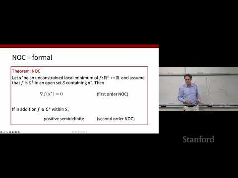
21:38 Necessary Optimality Conditions Theorem (NOC)

For an unconstrained local minimum x* of a C¹ function f within an open set:
1. ∇f(x*) = 0
2. If f is C², then H(x*) is positive semi-definite.

22:38 The Importance of Open Sets and Boundaries

NOC applies to points strictly within the domain, not on boundaries.
A local minimum on a boundary might not have a zero derivative.
Example: minimum of f(x) = x on [0, 1] is at x=0, but f'(0) = 1 ≠ 0.

27:28 Sufficient Condition for Optimality: Hessian Positive Definite

If ∇f(x*) = 0 and H(x*) is positive definite, then x* is a strict local minimum.
Positive definite Hessian implies the function locally behaves like a 'bowl' around x*.
This condition guarantees that any small perturbation increases the function value.

30:38 Convex Functions and Their Optimization Properties

Convex domain: line segment between any two points in the set is contained within the set.
Convex function: the line segment connecting any two points on the graph lies above or on the graph.
For convex functions, any local minimum is also a global minimum.

37:04 Optimization Benefits of Convexity

Local minimum of a convex function is a global minimum.
If f is strictly convex, there's at most one global minimum.
For differentiable convex functions, ∇f(x*) = 0 is both necessary and sufficient for global optimality.

40:50 Computational Methods: Gradient Descent

Iterative methods generate a sequence of guesses x₀, x₁, x₂, ...
Goal: ensure f(x₀) > f(x₁) > f(x₂) ... to approach a minimum.
Update rule: x_{k+1} = x_k - α * ∇f(x_k), where α is the step size.

57:25 Choosing Descent Direction and Step Size (α)

Descent direction d must satisfy ∇f(x)ᵀ d < 0.
Common choices for d: -∇f(x) (gradient descent) or -H(x)⁻¹∇f(x) (Newton's method).
Step size α can be fixed, determined by minimization, or diminishing (sum of α_k = ∞, α_k → 0).

1:05:49 Convergence Guarantees and Termination Criteria

Convergence to stationary points (∇f = 0) requires specific conditions on α and d.
Termination rules: fixed number of iterations, or |f(x_{k+1}) - f(x_k)| < ε.
Convergence rate (linear, superlinear, quadratic) depends on algorithm and function properties.

Summary, takeaways, and chapters were generated by AI from the video's transcript and may contain errors. The video belongs to its creator, Stanford Online.