Stanford AA203 Optimal and Learning-Based Control | Spring 2026 | Lecture 18: RL Policy Optimization

Overview

This lecture introduces policy optimization as a model-free reinforcement learning method, contrasting it with value-based approaches. It details the derivation of policy gradients, leading to the REINFORCE algorithm, and discusses variance reduction techniques like baselines. The session culminates in an explanation of actor-critic methods, which combine policy gradient and value-based learning to improve sample efficiency and stability, exemplified by the AlphaGo system.

Key takeaways

Policy optimization directly learns a parameterized policy by optimizing an RL objective using gradient ascent, unlike value-based methods which infer policies indirectly.
The REINFORCE algorithm is a foundational policy gradient method that uses Monte Carlo returns, but suffers from high variance.
Variance in policy gradients can be reduced by incorporating causality (reward-to-go) and using baselines, such as the average return or a learned value function.
Actor-critic methods combine the direct policy learning of policy gradients with the variance reduction capabilities of value function estimation (critic).
The advantage function, A(s, a) = Q(s, a) - V(s), is a key component in actor-critic methods, quantifying the benefit of a specific action over the average.
AlphaGo successfully employed an actor-critic architecture, using policy gradients with a value function baseline and guiding Monte Carlo Tree Search.

Chapters

0:06 Introduction to Policy Optimization in RL

Shifts from value-based methods to policy optimization within model-free RL.
Policy optimization explicitly represents and tunes policy parameters.
Goal is to directly maximize the reinforcement learning objective.

0:21 Reinforcement Learning Formalism: MDPs and Trajectories

Reinforcement learning agent interacts with an environment.
Trajectories are sequences of states and controls.
Formalized as a Markov Decision Process (MDP) with stochasticity from initial state, policy, and transitions.

0:47 Parametric Policy Representation

Policy is represented as a parametric function, pi(theta).
RL objective and trajectory distribution depend on policy parameters theta.
Optimization aims to find theta that maximizes the RL objective.

10:14 Gradient Ascent for Policy Optimization

Policy optimization uses gradient ascent to maximize the RL objective.
Requires estimating the gradient of the objective function.
Learning the policy becomes an iterative process of gradient descent on the objective.

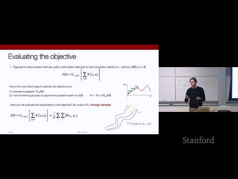
12:06 Estimating the Objective Expectation via Sampling

The RL objective involves an expectation over trajectory distributions.
This expectation is approximated by sampling multiple trajectories (rollouts).
Empirical mean of rewards from sampled trajectories approximates the expected return.

15:18 Deriving the Policy Gradient

Objective function J(theta) is the expected sum of rewards.
Gradient of J(theta) is derived using calculus.
Initial gradient expression depends on unknown environment dynamics.

20:02 Log-Derivative Trick for Policy Gradient

Uses the identity: p * grad(log p) = grad(p).
Transforms the policy gradient to involve grad(log pi).
Resulting expression is an expectation under the trajectory distribution of (grad log pi) * R(tau).

23:23 Decomposing the Log-Probability of Trajectories

Log of trajectory distribution factors into log initial state, log policy, and log transitions.
Gradient with respect to theta only affects the log policy term.
This isolates the policy's contribution to the gradient.

27:08 Actionable Policy Gradient Expression

The derived policy gradient is an expectation of (grad log pi) * R(tau).
All terms within the expectation are now known or computable.
Approximated by empirical mean over sampled trajectories.

30:26 The REINFORCE Algorithm

First policy optimization algorithm derived from the policy gradient.
Steps: sample trajectories, estimate policy gradient, update policy parameters.
Uses Monte Carlo estimation of returns (sum of rewards).

34:12 Intuition Behind Policy Gradients

Policy gradient updates probabilities of actions based on their performance (rewards).
Compares to Maximum Likelihood Estimation (MLE) / Behavior Cloning.
Policy gradient is a weighted version of MLE gradient, weighted by return.

45:53 High Variance in Policy Gradient Estimators

Policy gradient estimates can have high variance due to sampling noise.
This leads to unstable learning signals, slower convergence, and potential non-convergence.
Research in policy optimization focuses on reducing this variance.

54:13 Variance Reduction: Causality and Baselines

Strategy 1: Incorporate causality by summing rewards from current time step onwards (reward-to-go).
Strategy 2: Introduce baselines (b) by subtracting a constant from returns.
Subtracting a baseline does not change the expected gradient (unbiased estimator).

1:08:26 Baselines and Average Return

A common baseline is the average return over sampled trajectories.
Centering returns with a baseline encourages increasing probability of above-average behaviors.
Baselines significantly improve sample efficiency and stability.

1:12:03 On-Policy Nature of Policy Gradients

Policy gradient methods, as derived, are on-policy.
Require samples collected under the current policy to estimate the gradient.
Can be sample inefficient due to discarding old data.

1:15:35 Pros and Cons of Policy Gradient Methods

Pro: Naturally handle continuous action spaces.
Pro: Directly optimize the RL objective.
Con: On-policy nature can lead to sample inefficiency.

Summary, takeaways, and chapters were generated by AI from the video's transcript and may contain errors. The video belongs to its creator, Stanford Online.