2NM4 Week 4: Interpolation and curve-fitting
Overview
The lesson distinguishes exact interpolation from best-fit curve fitting, then develops polynomial and cubic-spline interpolation before extending the same linear-system framework to radial basis functions (RBFs). It connects Vandermonde matrices and Runge oscillations to practical alternatives, explains least-squares fitting with the pseudo-inverse and NumPy's polyfit, and shows why weights, measurement uncertainty, units, and model complexity matter when choosing a fit.
Key takeaways
- Exact polynomial interpolation through n + 1 distinct points requires a degree-n polynomial, but high-degree fits can oscillate between data points through the Runge phenomenon.
- Cubic splines control oscillation by fitting local cubics with C1 and C2 continuity; assembling the constraints produces a sparse, banded linear system.
- RBF interpolation handles scattered data in n dimensions by solving for weights on distance-based kernels, with kernel choice and epsilon controlling each point's spatial influence.
- Least squares can fit a lower-degree model to more observations by minimizing residuals through a rectangular system and pseudo-inverse, commonly computed with singular value decomposition.
- A smaller residual norm is not enough to choose model complexity: higher-degree polynomials can fit measurement noise, so the fitted trend and stability should inform degree selection.
- Weighted fits depend on measurement scale and reliability; consistent units and correctly interpreted uncertainty weights prevent one equation or measurement from dominating the result.
Chapters
- Interpolation passes through every data point and assumes distinct x-values with no measurement error.
- Curve fitting seeks a global trend, can accommodate repeated x-values with different y-values, and does not need to match every observation.
- Historical interpolation methods prioritized fast updates when new measurements arrived, a concern illustrated by the Babbage difference engine.
- A unique polynomial of degree n passes through n + 1 distinct data points, so 10 points determine a ninth-degree polynomial.
- Polynomial bases are easy to evaluate, differentiate, integrate, and manipulate algebraically.
- The interpolation error grows with the distance from the query point to the sampled points, making extrapolation especially risky.
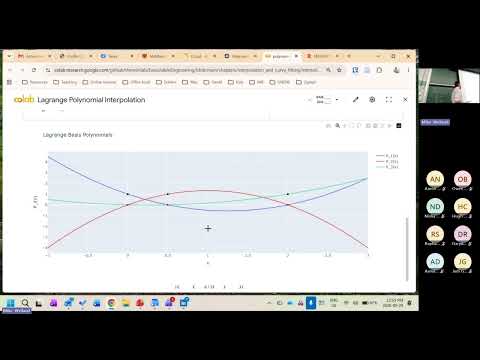
- Lagrange interpolation represents the result as a weighted sum of basis polynomials, each equal to 1 at its own data point and 0 at the others.
- That construction makes each basis weight equal to the corresponding measured y-value.
- With three data points the basis functions are quadratic; adding a fourth point produces cubic basis functions.
- Directly rebuilding and evaluating Lagrange products costs roughly O(n²), and adding a data point requires recomputing the construction.
- Barycentric Lagrange interpolation factors reusable terms to reduce repeated evaluation work.
- Newton divided differences produce the same polynomial while allowing a new observation to be added as another diagonal in a divided-difference tableau.
- Writing a polynomial in monomials turns coefficient estimation into a linear system whose rows contain powers of each sampled x-value.
- The resulting Vandermonde matrix is dense and notoriously ill-conditioned, so small numerical errors can greatly affect the fitted coefficients.
- When there are more data points than polynomial coefficients, the system becomes rectangular and can be treated as a least-squares problem.
- A tenth-degree interpolant through 11 points can oscillate sharply between observations, an effect known as the Runge phenomenon.
- Increasing polynomial degree can make these high-frequency oscillations worse, even inside the sampled interval.
- Cubic splines use separate low-degree polynomials over neighboring intervals to avoid the instability of one high-degree global polynomial.
- Cubic splines match the data at interval endpoints and enforce continuous first and second derivatives, or C1 and C2 continuity.
- Formulating all interval constraints together yields a sparse, banded linear system rather than a dense Vandermonde system.
- The resulting structure is well suited to sparse and iterative solvers, while local cubics reduce Runge-style oscillation.
- Radial basis functions generalize interpolation to multiple dimensions by defining each kernel through Euclidean distance from a data point.
- The interpolant is a weighted sum of kernels, but overlapping kernels mean the weights must be solved for simultaneously.
- Evaluating each kernel at each data point constructs a linear system, returning the method to the same linear-algebra framework as polynomial fitting.
- For kernels normalized to 1 at their centers, the RBF system has ones on its diagonal and typically smaller off-diagonal entries.
- Symmetry, diagonal dominance, sparsity, and banded structure can arise depending on the kernel and point arrangement.
- A small system can be solved with ordinary LU; a symmetric positive-definite system can use conjugate gradient, while sparse structure can support more scalable methods.
- Gaussian, inverse-quadratic, and inverse-multiquadratic kernels differ in how quickly their influence decays with distance.
- The tuning parameter epsilon controls kernel width; average spacing between data points is offered as a practical starting estimate.
- RBFs can fit two-dimensional surfaces from scattered samples, though randomized sampling can produce notably different interpolation quality.
- Multivariate polynomials can develop Runge-like behavior rapidly as products of powers in x and y increase in complexity.
- Nearest-neighbor and linear interpolation are alternatives, but unstructured points require triangulation to determine which observations influence a query.
- RBFs work in n dimensions and avoid requiring a preselected polynomial shape, making them a flexible basis for scattered data.
- A cubic has four coefficients, so fitting it to 10 observations produces a rectangular system with no exact solution in general.
- Least squares minimizes the residual norm, and the pseudo-inverse provides a general solution for rectangular matrices, typically computed through singular value decomposition.
- When the system is square and invertible, the pseudo-inverse reduces to the ordinary inverse and the exact solution is also the least-squares solution.
- NumPy polyfit estimates polynomial coefficients using a least-squares approach based on the Vandermonde system.
- The example adds Gaussian noise to a known fourth-order polynomial and compares fits of different degrees.
- A 50-point, 50th-degree interpolant could match every noisy observation, but exact agreement would overfit noise and risk severe oscillation.
- Residual norm generally decreases as polynomial degree rises, so minimizing that quantity alone does not identify a useful model.
- The true fourth-degree example does not necessarily have its lowest residual at degree four because higher-degree fits can absorb noise.
- A practical engineering judgment is to prefer the lowest degree whose fitted shape remains stable as higher degrees are tried.
- Weighted least squares changes how strongly each equation influences the fit; multiplying one equation by 10 can pull the solution toward that observation.
- Measurement repeatability can guide weights: readings clustered near 50, such as 49, 50, and 51, are more reliable than highly variable readings such as 100, 200, and 300.
- Use consistent units, comparable scales, or logarithms where appropriate, and check whether a library expects variance, standard deviation, or an inverse quantity as its weight.
- An RBF fit can use fewer kernels than observations, such as 10 kernels for 100 data points, and SciPy methods can combine RBFs with a low-order polynomial to preserve global trends.
Transcript excerpt
0:00 I'm going to move on. Interpolation and curve fitting. Uh I got to speed through this a little bit to make up for uh tomorrow's uh tomorrow's skipping. Okay. Um in both cases, what we're going to do is we're going to get a whole set of data and we're going to be asking like what is the general function interpolation and curve fitting kind of differ in that interpolation typically go through all of those data points and you want to know like given these data points, what is the value in between those? Right? you're interpolating between those guys. Um, typically you assume that there is no measurement error. If you have one guy here, another guy here, another guy here, you're going to fit a curve that roughly goes through all those guys. You're not going to do any kind of averaging. Um, there's no ambiguity in X and Y. There's no like duplicate X values, different Y values
0:48 for the same X. Um, typically they capture local behavior as opposed to curve fitting. Right? The magic's in the name fitting. It calculates the best fit for the data points. Doesn't necessarily traverse and match all of those individual data points, but it will give you kind of the general trend, right? Um, you can have ambiguity in XY pairs. You can have two values of X and different values in Y. It is more intended to be a global encapsulation of the data. Um, generally speaking, it is the generalization of interpolation. If you drill down the curve fit to the point where it has to be exact, right? Typically, you'll have a parameter, you have to be exact, then you will recover the interpolation. Does this sound
1:35 familiar to anybody who was here on Friday and learned about the pseudo
This is the start of the transcript. Save this video free for the whole transcript, searchable and time-coded.
In this course
Related notes
Summary, takeaways, and chapters were generated by AI from the video's transcript and may contain errors. The video belongs to its creator, Numerical Methods for Engineering.