2NM4 Week 2: Linear systems (direct)
Overview
The lecture develops direct methods for solving linear systems, connecting solvability and conditioning to matrix norms, sparsity, and computational cost. It explains Gaussian elimination, pivoting, diagonal dominance, and LU or PLU factorization, emphasizing that dense factorization scales as O(n^3), sparse structure can reduce costs, and reusable factors are preferable to explicitly forming A inverse.
Key takeaways
- For a square system, a nonsingular coefficient matrix gives a unique solution; a singular matrix may yield either no solutions or infinitely many, depending on b.
- The condition number κ(A) = ||A|| ||A inverse|| captures worst-case sensitivity, and a spectral condition number equals the largest singular value divided by the smallest.
- Dense Gaussian elimination costs approximately N cubed divided by 3 operations, while back substitution costs O(N^2); increasing matrix size by a factor of 10 can therefore multiply dense elimination work by about 1,000.
- LU factorization separates a system's coefficient matrix from its right-hand side, allowing one O(N^3) factorization to be reused for multiple b vectors.
- Sparse storage and sparse solvers can greatly reduce memory for structured systems, but fill-in during LU and density of an explicitly formed inverse can erase those gains.
- Zero or tiny pivots can break elimination or magnify roundoff; row permutations select safer pivots, while strict diagonal dominance provides a useful structural guarantee.
Chapters
- A linear system is written as A x = b, where A contains coefficients, x contains unknowns, and b contains constants.
- The lecture distinguishes linear expressions such as a x from nonlinear examples such as x squared, square root of x, and x y.
- For an M by N coefficient matrix, x has length N and b has length M; square systems have M = N.
- Before selecting a solver, determine whether a system has a solution and whether that solution is unique.
- Matrix norms measure matrix size or transformation strength, while conditioning describes how input uncertainty affects outputs.
- Finite-precision roundoff introduces numerical error, and sparsity can make large matrix computations practical.
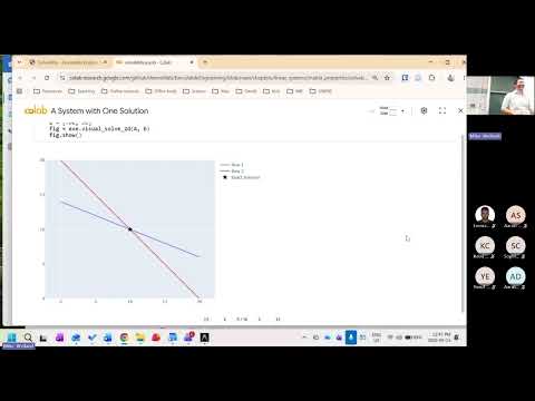
- The example uses chairs costing $20, tables costing $50, a $700 budget, and space for 20 items.
- The equations 20C + 50T = 700 and C + T = 20 intersect at C = 10 and T = 10.
- Each equation describes a line of possible values, and their intersection satisfies both equations simultaneously.
- Multiplying the item-count equation by 20 and subtracting eliminates the chair variable, leaving 30T = 300.
- For a 2 by 2 matrix, the determinant is ad minus bc; a nonzero determinant allows an inverse and a unique solution.
- Directly computing a general matrix inverse becomes cumbersome as matrix size grows, motivating algorithmic solution methods.
- If chairs and tables both cost $20 and the budget is $400, the two equations coincide, producing infinitely many solutions.
- Changing the budget to $500 makes the equations parallel and inconsistent, so no solution exists.
- Both cases have a singular coefficient matrix; singularity rules out a unique solution but does not alone determine whether solutions are absent or infinite.
- Two equations in two unknowns represent lines; in three dimensions, equations represent planes.
- Independent rows describe distinct constraints, while dependent rows can produce either coincident constraints or inconsistent ones.
- A consistent system has at least one solution, even when that solution is not unique.
- The L2 norm is the Euclidean length, computed by taking the square root of the sum of squared vector components.
- The L1 norm sums absolute component values and corresponds to Manhattan distance on a grid, such as a 3-block by 10-block route.
- The infinity norm is the largest absolute component, obtained as the limit of increasingly high-power norms.
- An induced matrix norm measures the greatest stretching of any unit vector under a matrix transformation.
- The spectral norm is the maximum stretch, equal to the largest singular value; the Frobenius norm and infinity norm offer easier-to-compute alternatives.
- Applying a matrix to the unit circle produces an ellipse, making the transformation's maximum and minimum stretches visible.
- As two equation lines approach coincidence, their intersection becomes highly sensitive to small changes in coefficients.
- The example changes a table price from 20 to 20 minus epsilon; the exact solution grows dramatically as epsilon approaches zero.
- Roundoff and subtractive cancellation can prevent finite-precision computation from distinguishing nearly coincident lines.
- A well-conditioned transformation preserves enough separation between data points for numerical computations to distinguish them.
- A uniform scaling, such as multiplying by 2, can be well-conditioned because its inverse scales by one-half and reverses the change.
- Ill-conditioned matrices squeeze some directions and stretch others, so reversing the transformation does not eliminate the worst-case sensitivity.
- The condition number is κ(A) = ||A|| ||A inverse|| and bounds worst-case relative error between x and b.
- For the spectral norm, the condition number is the ratio of the largest to smallest singular value.
- A condition number of 1 is ideal; the identity matrix is the reference case because it leaves vectors unchanged.
- Zero, identity, diagonal, upper-triangular, lower-triangular, and symmetric matrices have distinct structures useful to solvers.
- A symmetric positive definite matrix corresponds to an upward-curving quadratic bowl; a saddle has curvature of opposite signs in different directions.
- For an orthogonal matrix, the inverse equals the transpose.
- Sparse matrices contain many zeros, often in a recognizable pattern that can reduce storage and computation.
- Finite-element systems commonly produce structured sparse matrices, including patterns with diagonal blocks.
- For large systems, such as matrices around 1,000 by 1,000 or larger, sparse storage can save substantial memory.
- A banded matrix has nonzero entries concentrated near its main diagonal; tridiagonal systems have one neighboring diagonal on each side.
- One-dimensional finite-difference heat or transport problems commonly produce tridiagonal matrices, while multidimensional dependencies widen the band.
- Block and block-diagonal structures can be exploited in multiphysics solvers, including segregated solution strategies.
- For an N by N matrix, Big O notation describes how operation counts scale as N grows, focusing on the highest-order term.
- Standard matrix multiplication takes O(N^3): it computes N squared output entries, each using an N-length dot product.
- Strassen's algorithm reduces the matrix-multiplication exponent to about 2.81, though the lecture focuses on conventional costs.
- The example profiles matrix multiplication on random matrices of increasing size and compares measured times with an N cubed curve.
- Matrix addition, transpose, and common matrix norms scale as O(N^2), while dense matrix inversion typically scales as O(N^3).
- Big O helps compare scaling, but parallel architectures such as GPUs and high-performance computing also affect real execution time.
- Gaussian elimination applies row operations to transform A x = b into U x = b prime, where U is upper triangular.
- Back substitution solves the resulting system from the last unknown upward and takes O(N^2) operations.
- The row operations preserve the solution while changing matrix properties such as its norm and condition number.
- An augmented matrix appends b to A so row operations can be applied to coefficients and constants together.
- Each elimination step uses a pivot entry to remove entries below it, producing an upper-triangular system.
- The example tracks elimination multipliers, which later become the entries of the lower-triangular factor in LU decomposition.
- The elimination phase costs approximately N cubed divided by 3 operations, so dense direct solving scales as O(N^3).
- Gauss-Jordan elimination also removes entries above the diagonal, but its leading operation count is about N cubed divided by 2.
- Because Gauss-Jordan costs more overall than Gaussian elimination plus back substitution, it is usually not the preferred numerical method.
- A zero pivot causes division by zero during elimination, even when reordering the equations would leave the system solvable.
- Row swapping, represented by a permutation matrix, moves a more suitable pivot into position.
- A pivot near machine precision can amplify roundoff, so choosing a larger pivot improves numerical stability.
- A matrix is strictly diagonally dominant when each diagonal entry's absolute value exceeds the sum of the other absolute values in its row.
- Diagonal dominance helps ensure pivots are not zero or dangerously small and can eliminate the need for beneficial row permutations.
- The property also becomes relevant to the convergence and analysis of iterative methods.
- LU factorization writes a square matrix as A = L U, with L lower triangular and U upper triangular.
- The elimination multipliers form the entries below L's diagonal, which is conventionally filled with ones.
- Multiplying L and U reconstructs the original matrix, while triangular structure enables forward and backward substitution.
- LU decomposition is not unique unless additional conventions constrain the factors; rescaling L and U can preserve their product.
- Factorization depends on A, not on b, so the same factors can solve multiple systems with different right-hand sides.
- After factorization, each new right-hand side needs triangular solves rather than repeating the full O(N^3) elimination.
- Sparse factorization can exploit the original matrix's structure, but fill-in may create new nonzero entries during elimination.
- Explicitly forming A inverse can turn a sparse tridiagonal matrix into a dense matrix, increasing storage from roughly O(N) to O(N^2).
- Storing L and U and using forward and backward substitution preserves opportunities to exploit sparsity.
- Optimized libraries such as NumPy and SciPy provide direct solvers; sparse input must use a sparse representation to activate sparse routines.
- For an N by N tridiagonal matrix, sparse storage needs roughly 3N values, while a dense representation needs N squared entries.
- Direct solvers are a robust default for many problems, but large dense solves can exhaust RAM; test small systems before scaling up.
- The lecture notes that some libraries can return least-squares-style solutions for singular systems, so users must verify what problem the solver actually solved.
Transcript excerpt
0:00 linear solvers. Uh the whole art and science of numerical methods is going to be boiling things down and down and down and down to the point where it is trivial. Trivial on this level in this course means linear systems, right? Linear systems you guys should know at this point, but it's it's like for example the canonical solve, right? Anything that can be expressed as ax plus minus b is a linear transformation. A linear system looks like this. Solve for x is equal to b over a. Is anybody confused about this? Okay, good. In contrast, x^2 is nonlinear, right? Anybody know why that's nonlinear? It isn't a straight line on a graph. It
0:50 is quite literally like a line. Linear like a line, right? Specifically, it is the factor that you actually multiply these guys, right? There are transformation rules. There is like the mathematical definition of linearity. We're we're just kind of put that under there and like move on with our lives. I really like the line on a graph. Um s of x linear or no? No. Uh how about square root of x? Anybody think that's linear? Put up your hand. No. Right. Anything like that. How about x y? Is that linear in xy? Whoever thinks yes, keep your hand down. If you think no, raise your hand up. Good. We got some exercise. It is not linear. Technically, I think it's called bilinear, but we're we're not even going there. It is not linear for our purposes. It is not linear. Okay.
1:39 More complicated example is when you have multiple equations and unknowns. Ax plus b y is equal to e. I'm sorry about the repeating b and b there. blah blah blah. This is called a linear system. Do
This is the start of the transcript. Save this video free for the whole transcript, searchable and time-coded.
In this course
Related notes
Summary, takeaways, and chapters were generated by AI from the video's transcript and may contain errors. The video belongs to its creator, Numerical Methods for Engineering.