CPBS 7620 - Lecture 17 - Linear Dynamical Systems

Overview

Nicholas Dwork defines continuous and discrete linear dynamical systems, then shows how forward Euler discretization turns continuous state equations into a form whose outputs are affine functions of the inputs. By stacking those input-output relationships into matrices, control becomes a least-squares problem; a two-compartment lung model demonstrates setting ventilator pressure to reach a target tidal volume or follow a desired trajectory.

Key takeaways

Forward Euler discretization converts x′(t) = A(t)x(t) + B(t)u(t) into a stepwise update with A_D = I + AΔt and B_D = BΔt.
For a discrete linear system, repeatedly substituting the state update expresses each output as an affine function of the initial state and the full sequence of prior inputs.
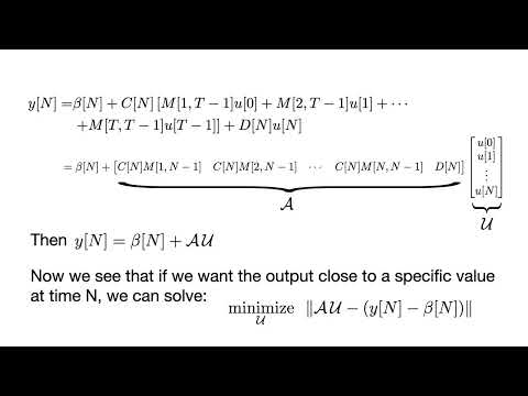
A desired terminal output can be written as yₙ = βₙ + 𝒜u, making input selection a least-squares optimization rather than an ad hoc control procedure.
The two-compartment lung model captures differing resistance and compliance across lung regions while predicting the ventilator’s measured total volume as V₁ + V₂.
In the ventilation example, a 0.2-second control interval over one second yields five pressure inputs, U₀–U₄, that can be optimized for a 0.45 L target tidal volume.
Least squares can target an entire output trajectory, such as a linear ramp to 0.45 L, by minimizing summed squared deviations at intermediate time steps.

Chapters

0:00 State, Input, Output, and Euler Discretization

A continuous linear system uses x′(t) = A(t)x(t) + B(t)u(t) and y(t) = C(t)x(t) + D(t)u(t); x is the state, u the chosen input, and y the output.
A, B, C, and D are respectively the dynamics, input, sensor, and feed-through matrices, and may vary with time.
Using a first-difference approximation with step size Δt gives x(t + Δt) ≈ [I + A(t)Δt]x(t) + B(t)Δt u(t), a discrete-time state update.
Indexing time as tₙ = nΔt yields a discrete system that approximates the continuous dynamics when Δt is sufficiently small.

2:50 Unrolling the Discrete System into a Least-Squares Control Problem

Repeatedly substitute the state update to express outputs such as y₁, y₂, and y₃ in terms of the initial state and all inputs up to that time.
Products of dynamics matrices describe how earlier states and inputs affect later outputs; stacking terms produces a block-matrix relation yₙ = βₙ + 𝒜u.
The resulting affine input-output map lets a desired output be pursued by solving a least-squares problem for the input sequence.
For a trajectory rather than one endpoint, stack the output errors across time and minimize their summed squared L₂ norms.

5:09 Two-Compartment Lung Model for Ventilator Pressure Control

The lung model has two compartments, each with its own airflow resistance Rᵢ and compliance Cᵢ; the compartments represent different mechanical behavior, not anatomically separated regions.
Ventilator input u(t) is airway pressure above PEEP, with about 8 cm H₂O given as a reasonable adult PEEP; measured output is total lung volume V₁ + V₂.
With pressure updates every 0.2 seconds, the continuous model is discretized into xₖ₊₁ = Axₖ + Buₖ and yₖ = Cxₖ; reaching one second requires choosing U₀ through U₄.
Starting at end-expiration with x₀ = 0, Dwork forms y₅ = GU and uses the pseudoinverse-based least-squares solution to target 0.45 L, or to fit a linear ramp toward that volume.

Summary, takeaways, and chapters were generated by AI from the video's transcript and may contain errors. The video belongs to its creator, Nicholas Dwork.