STAT 3011 Fall 2026: Sampling distribution of Means
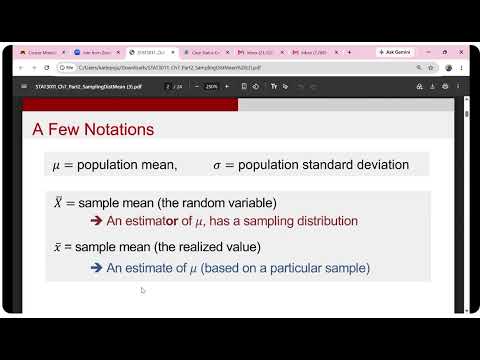 Watch on YouTube →
Overview
Prof Kazeem Adepoju explains the sampling distribution of the sample mean, contrasting samples from normal populations with samples from skewed or other non-normal populations. He develops the standard error formula, σ/√n, and the Central Limit Theorem rule used in class that independent random samples of at least 30 observations have an approximately normal sampling distribution, then applies the ideas to TV-watching, soda bottles, and household-size examples.
Key takeaways
- The sampling distribution of X-bar is centered at the population mean, so the sample mean is an unbiased estimator when observations are selected through an appropriate random sampling process.
- For independent observations, the standard error of the sample mean is σ/√n; increasing n narrows the distribution of sample means without changing its center.
- If the population is normal, the sampling distribution of X-bar is normal for any sample size; if the population is non-normal, this class uses n ≥ 30 as a rule of thumb for approximate normality with independent observations.
- A non-normal individual variable can still have an approximately normal sample mean: the number of children per household is discrete, but a random sample of 50 households supports a normal approximation for X-bar under the class's Central Limit Theorem rule.
- Probability questions about a single observation use the population standard deviation, whereas probability questions about a sample average use the standard error σ/√n.
- For the household example with σ = 1.68 and n = 50, the standard error is approximately 0.238; for the TV example with σ = 2.25 and n = 100, it is 0.225.
Chapters
- Prof Kazeem Adepoju announces that Exam One practice questions are posted and that Wednesday's class will review them rather than begin a new topic.
- The Wednesday review will be recorded and shared by Zoom link, with information about exam coverage and what students should bring.
- Adepoju briefly mentions an optional birthday event planned for October 31.
- A study of University of Minnesota students' weekly food spending could produce different averages across investigators, even when each uses the same sample size.
- A sampling distribution describes the possible values of a statistic, such as a sample mean, and their probabilities across repeated samples.
- Random selection is presented as the way to make the sample mean an unbiased estimate of the population mean.
- For a normal population with mean 50 and standard deviation 10, the sampling distribution of X-bar remains normal for sample sizes such as 2, 10, and 100.
- As sample size increases, the sampling distribution's center remains at the population mean while its spread decreases.
- Adepoju connects convergence of sample averages to the population mean with Jacob Bernoulli's Law of Large Numbers and cites Abraham de Moivre's 1733 work on normal approximation to the binomial.
- A skewed population can produce a skewed sampling distribution when the sample size is small, while larger samples make the distribution of X-bar more bell-shaped.
- The class rule is that for independent observations from a non-normal population, n at least 30 supports an approximately normal sampling distribution.
- For a binomial random variable, the population mean is np and the standard deviation is √(np(1-p)); repeated sampling illustrates how the sampling distribution can approach a normal shape.
- The standard deviation of individual observations, σ, differs from the standard deviation of the sample means, σX-bar, also called the standard error.
- For independent observations, the standard error is σ/√n; it equals σ when n = 1 and becomes smaller as n increases.
- Adepoju summarizes that the expected value of X-bar is the population mean, while increasing sample size reduces the variability among sample means.
- Daily TV-watching hours are modeled with population mean 3 hours and standard deviation 2.25 hours, and the supplied population graph is skewed.
- For a sample of 10 Americans, σ/√n can be calculated, but the class's n ≥ 30 rule does not support assuming normality for this skewed population.
- For a sample of 100, the Central Limit Theorem supports an approximately normal distribution of X-bar, with standard error 2.25/√100 = 0.225 hours.
- To find a sample size that makes the standard error no greater than a target, start from σ/√n ≤ target.
- Rearranging gives n ≥ (σ/target)², so the required sample size depends on both the population standard deviation and the desired precision.
- Adepoju assigns students to use this relationship for a standard-error target of 0.1.
- The first soda example asks for the probability that one bottle contains less than its 295 ml label amount, using the population's normal model.
- A second question concerns the average amount in a randomly selected six-pack, so the target becomes P(X-bar < 295).
- For six bottles, the mean remains the population mean while the standard deviation for X-bar is σ/√6; normality is justified because the bottle-fill population is stated to be normal, not because n reaches 30.
- The number of children per U.S. household has mean 1.90 and standard deviation 1.68, but the individual variable is not normally distributed because it is discrete and cannot be negative.
- For a random sample of 50 households, the class applies the Central Limit Theorem because n exceeds 30 and the sample is random, giving X-bar an approximately normal distribution.
- The standard error is 1.68/√50, approximately 0.238 children; this is used to calculate the probability that the sample average exceeds 3.
- Adepoju sets up the household example as P(X-bar > 3), using the sample-mean distribution's mean of 1.90 and standard error of 1.68/√50.
- In R's pnorm function, the upper-tail option is set to FALSE for the greater-than probability; the lower-tail setting is used for a less-than probability.
- The class closes with a reminder to stay safe.
Transcript excerpt
0:04 But then it just stopped working. It just don't She should have heated up Well, naturally >> Okay.
2:08 Uh Good morning, everyone. I want to welcome you to another statistical analysis class. Uh those of you at the back, uh can you hear me? Okay. Thank you so much. Thank you for confirming that. Uh before I get started today, I have announcement to make. Number one, I've posted exam one practice question for this uh semester. Uh of course, uh today we're going to go over the last topic before the midterm. And I'm advising every one of you to be around
2:54 on Wednesday. On Wednesday, we never we're not going to start a new topic. We only going to uh go over the midterm one practice, and I'm also going to give you information about um you know, the exam. You know, what you need to bring into the exam, what are the areas the exam will cover, and so on like that. So, and and it's also going to be recorded. Okay, the one on Wednesday will be recorded. I'm not going to put it on YouTube, but I'm going to share the Zoom link for the one for Wednesday, because it is centered on reviewing exam one. Uh the last announcement before I get started. You know, some of you
3:42 have been reaching out. Uh you saw a video on YouTube that has to do with my birthday preparation, and uh you want to know what is going on. So, I think I'm quickly going to tell you this. My birthday is coming up and I don't want to disturb you because you have a lot, okay? Um the birthday is going to take place on October 31st. Okay? If you have If you If If you have
This is the start of the transcript. Save this video free for the whole transcript, searchable and time-coded.
Related notes
Summary, takeaways, and chapters were generated by AI from the video's transcript and may contain errors. The video belongs to its creator, Prof Kazeem Adepoju.