Section 4.5 Lecture (Part 1): Inference with Regression Models
Overview
Brad Hall explains regression inference by distinguishing the overall F test of joint significance from t tests of individual predictors, then demonstrates both with Excel output. In the coffee-shop model, the three predictors are jointly significant; in the 2025 NFL example, the model is jointly significant, but field-goal percentage is not individually significant at 5%, prompting a comparison of separate R-squared values for offensive and defensive yards per play.
Key takeaways
- For a regression model with several predictors, the joint F test addresses whether all slopes are zero, while individual coefficient tests determine which predictors contribute after accounting for the others.
- Excel's ANOVA output reports the overall F statistic and its p-value as Significance F; the coffee-shop model's F = 86.556 and p = 1.94 × 10⁻⁶ support joint significance at α = 0.05.
- A coefficient confidence interval that excludes zero indicates individual significance at its corresponding two-sided confidence level; the campus-sales interval in the coffee example is approximately $2,694 to $7,306.
- A significant overall model does not guarantee that every predictor is significant: the NFL model's joint p-value is about 5.85416 × 10⁻⁷, while field-goal percentage's individual p-value is 0.080.
- In separate NFL win-percentage regressions, offensive yards per play has R² = 36.49%, compared with 19.74% for defensive yards allowed per play.
Chapters
- The chapter recap moves from correlation between two numerical variables to simple and multiple linear regression.
- Dummy variables let categorical features such as a coffee shop's drive-through or campus location enter a regression model.
- Goodness-of-fit measures describe how closely a model fits observed data, but do not by themselves establish statistical significance.
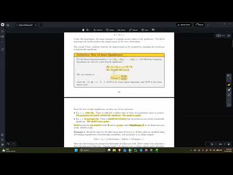
- The joint null hypothesis sets every predictor slope to zero; the alternative says at least one population slope is nonzero.
- Rejecting the null supports the conclusion that the predictors are jointly significant and the model is useful as a whole.
- The F statistic is the regression mean square divided by the error mean square, both drawn from the ANOVA table.
- In the coffee-shop example, the overall F statistic is 86.556 and Excel labels its joint-test p-value Significance F.
- The reported Significance F is 1.94 × 10⁻⁶, below α = 0.05, so the joint null hypothesis is rejected.
- Advertising, drive-through status, and campus proximity are jointly significant predictors of weekly sales in this model.
- An individual test evaluates one slope at a time while accounting for the other predictors in the model.
- A nonzero slope indicates evidence of a linear relationship between that predictor and the response, conditional on the other model variables.
- Excel's regression output reports two-tailed coefficient p-values; a one-tailed p-value can be obtained by halving the value when the coefficient's direction matches the stated alternative.
- The advertising test asks whether advertising has a positive linear relationship with weekly sales while the other predictors are held constant.
- Excel reports a two-tailed p-value of about 1.11937 × 10⁻⁶; the lecture halves it for the positive, one-tailed alternative.
- The resulting p-value is far below α = 0.01, supporting advertising as an individually significant positive predictor.
- The drive-through test compares shops with a drive-through, coded 1, against shops without one, coded 0, and asks whether the former have higher expected sales.
- Its reported p-value is about 3.6683 × 10⁻⁵; halving it for the one-tailed test still leaves it below α = 0.01.
- Excel's lower and upper 95% coefficient bounds provide another significance check: an interval that excludes zero indicates a nonzero slope at the corresponding two-sided level.
- The campus example uses the coefficient interval rather than the p-value to assess whether campus proximity predicts weekly sales.
- The stated 95% bounds correspond to an estimated weekly-sales effect from about $2,694 to $7,306, and the interval excludes zero.
- Because zero is outside the interval, the campus slope is statistically significant; the sales estimate can also inform a business owner's rent and return-on-investment decision.
- The 2025 NFL regular-season example models team win percentage using offensive yards per play, defensive yards per play, and field-goal percentage.
- Each team's win percentage is based on 17 games, with a tie counted as half a win.
- Brad Hall uses Excel Data Analysis Regression, selecting win percentage as Y and all three measures as the X range.
- The fitted equation has positive directions for offensive yards per play and field-goal percentage, and a negative direction for defensive yards allowed per play.
- The overall model's joint-test p-value is about 5.85416 × 10⁻⁷, well below α = 0.05.
- Rejecting the joint null supports the model as a whole, but does not establish that each of its three predictors is individually useful.
- For two-tailed individual tests at α = 0.05, the p-values for offensive and defensive yards per play round to 0.000.
- Field-goal percentage has a p-value of 0.080, which exceeds 0.05, so it is not individually significant in the three-predictor model.
- The result suggests field-goal percentage may be sharing explanatory information with the other predictors; possible next steps include removing it or measuring special teams more granularly.
- Brad Hall fits two simple regressions, each predicting win percentage from only one of the yardage variables.
- Offensive yards per play has R² = 0.3649, explaining about 36.49% of the observed variation in win percentage in its separate model.
- Defensive yards per play has R² = 0.1974, or about 19.74%; the lecture concludes that the offensive measure explains more variation in this comparison.
Transcript excerpt
0:01 Hey everyone. This is section 4.5 on inference with regression models. So this is the last section not only in this module, which is module six and also the last section in unit three. This is also the final section for all of the lecture material for ISDS 2001. So here we will conclude with some of the techniques that we use for regression analysis, in particular linear regression analysis by ultimately testing the way in which we can discover and apply statistical significance to not only our models as a whole, but the
0:50 predictors on an individual level. So to briefly recap what what brings us here. So remember throughout this chapter we started off trying to simply compare the correlation between two numerical variables. And so we had the correlation coefficient that we used to measure that. We then looked at this in terms of one of these being an input variable, known as a predictor variable, and then the other one being an output also known as a response variable and trying to see does this relationship form a linear relationship or any relationship at all. And so that was known as a simple regression
1:38 model or simple regression equations. And then we took that a step further by also introducing well maybe not just having one input or predictor variable, but why not two or three or four? And this brings us into multiple linear regression. And we also included dummy as well, which were ways of taking categorical variables, translating them to numbers, so that way we can actually use those in analyses as well. And finally, we talked about goodness of fit um goodness of fit measures in section 4.4 which helped us examine how well sample regression equations fit observed data.
2:28 Because remember, the the main point of
This is the start of the transcript. Save this video free for the whole transcript, searchable and time-coded.
In this course
Related notes
Summary, takeaways, and chapters were generated by AI from the video's transcript and may contain errors. The video belongs to its creator, Brad Hall.