Princeton Intro to Robotics (Fall 2026) | Lecture 13: Occupancy-Grid SLAM
Overview
The lecture develops occupancy-grid mapping from Bayesian filtering, first assuming a known robot pose and then relaxing that assumption to introduce Grid-based FastSLAM. Its central techniques are independent per-cell occupancy estimates, sensor likelihood updates, and particles that jointly represent robot pose and map, enabling loop closure when a robot revisits a location.
Key takeaways
- A grid with N binary occupancy cells has 2^N possible maps; treating cells as independent reduces the estimate to N separate occupancy probabilities.
- A range sensor updates only cells supported by its visible ray: cells before a return can be marked free, the hit cell occupied, and unseen cells left unchanged.
- Occupancy-grid Bayesian updates avoid summing over all 2^N maps by taking the ratio of occupied to free posterior probabilities, then using log odds for numerical stability.
- Grid-based FastSLAM stores a pose and map hypothesis in each particle, weights each joint hypothesis by sensor-measurement likelihood, and resamples accordingly.
- Loop closure can correct accumulated map drift when a robot revisits a location, but only if the particle set still includes a hypothesis near the true pose and map.
- Classical SLAM offers modular, interpretable components that are easier to debug, while its model assumptions can constrain accuracy and motivate learning-based alternatives.
Chapters
- The Kalman filter is an exact Bayesian filter when dynamics, sensor models, and the initial belief are linear and Gaussian.
- Particle filters support nonlinear, non-Gaussian models by approximating beliefs with a finite set of weighted samples.
- In known-map localization, particles represent pose hypotheses; a symmetric corridor can produce two clusters until room features distinguish the robot's location.
- A rangefinder model conditions measurement likelihoods on robot pose and map, using the expected distance to the nearest obstacle.
- Realistic range sensors can report the correct distance, a shorter false return, a spurious obstacle, or the maximum range when detection fails.
- Sensor-specific error probabilities must be characterized before applying a particle filter to LIDAR or ultrasound measurements.
- SLAM addresses the localization-mapping dependency: mapping needs a pose estimate, while localization needs a map.
- Geometric representations include occupancy grids, point clouds, and neural level sets such as a network's zero level set.
- Semantic maps add object and place meaning, supporting tasks such as finding a cup in a kitchen, while geometric maps support navigation.
- A 2D occupancy grid represents each cell as occupied or free; a 3D grid uses voxels.
- A grid with 30 cells is a 30-element binary vector, with 1 for occupied and 0 for free.
- Mapping estimates a probability distribution over maps from the robot's state history and sensor observations, allowing false-positive and false-negative sensor reports.
- A grid of N binary cells has 2^N possible maps, making a full joint distribution impractical even for modest grids.
- The naive Bayes assumption treats cell occupancies as independent, reducing the representation to N separate binary probabilities.
- Real environments violate strict independence because neighboring cells tend to share occupancy, but the approximation makes filtering computationally manageable.
- A prior can be set from expected occupancy; the lecture suggests roughly 10% to 20% occupied space for a typical room, rather than assuming every cell is equally likely.
- The occupancy update considers one cell at a time because the naive Bayes model treats cells independently.
- A binary measurement Z_i indicates whether the sensor reports cell i as occupied, abstracting real range readings into occupancy evidence.
- A range return can mark cells along the visible ray as free up to the hit and the hit cell as occupied.
- Cells outside the sensor's line of sight are generally left unchanged because the measurement provides no evidence about them.
- Bayes' rule combines the cell's prior occupancy probability with the likelihood of its sensor report given the robot pose.
- For cells other than the robot's current cell, the derivation approximates occupancy as independent of robot pose.
- The pose-independence approximation fails for the cell containing the robot, which must be free under the perfect-localization assumption.
- The update uses the sensor's false-positive and false-negative probabilities to assess how strongly a report should change occupancy belief.
- The normalizing likelihood can be expanded by summing over possible maps using the law of total probability.
- That direct calculation requires considering 2^N maps, the same exponential obstacle that makes a full map distribution infeasible.
- The derivation identifies this denominator as the expensive term and motivates a more efficient update based on comparing occupied and free probabilities.
- Dividing the posterior probability of occupancy by the posterior probability of being free cancels the difficult normalization term.
- The resulting ratio combines the prior odds with sensor likelihoods for the observed binary report.
- Because occupancy and free space are complementary outcomes, their probabilities sum to one, leaving a single probability to compute.
- Implementations commonly store log odds, the log of the probability ratio, to avoid numerical problems when probabilities approach 0 or 1.
- Per-cell Bayesian updates can run independently across all N cells and repeat as new measurements arrive.
- Occupancy-grid visualizations often threshold the underlying probability, for example marking cells occupied above 0.5.
- A drone's map can support trajectory planning, but real robots lack both a perfect map and perfect localization.
- Joint SLAM must estimate robot state and map together rather than treating either as known.
- Each Grid-based FastSLAM particle contains both a robot-pose hypothesis and its associated occupancy-map hypothesis.
- At each time step, particles propagate through the motion model and update their maps using occupancy-grid filtering.
- Importance weights measure how likely each particle's map and pose are to have produced the new sensor measurement.
- Resampling draws particles in proportion to their weights, retaining more plausible joint hypotheses and allowing duplicates.
- A map built while the robot moves can drift, producing implausible geometry such as a corridor that fails to meet a previously mapped wall.
- When the robot returns to a previously visited location, measurements can favor a consistent pose-and-map particle and pull the map back into alignment.
- This loop-closure effect depends on retaining enough diverse particles, including one close to the true pose and map.
- If resampling eliminates all particles near the correct hypothesis, the filter cannot recover it without mechanisms such as introducing new particles.
- Explicit loop-closure methods can compare current and past RGB images to determine whether they depict the same place.
- Feature correspondence must tolerate changes such as a car appearing in one image but not another or objects shifting position.
- Recognizing a revisited location adds evidence that can correct the accumulated pose and map estimate.
- An indoor drone can combine depth sensing, an inertial measurement unit, and optical flow when GPS becomes unreliable.
- The demonstrated system builds a 3D occupancy map while planning trajectories and exploring previously unseen regions.
- Classical Bayesian and particle-filter pipelines are modular and interpretable, making sensor-model and dynamics-model failures easier to debug.
- Their assumptions, including known models and independent grid cells, can limit performance; learning-based end-to-end methods are increasingly prominent, though classical stacks remain useful in deployed systems.
- Classical SLAM exposes components such as the sensor model and motion model, so engineers can test and improve them independently.
- The same pipeline depends on carefully chosen models and approximations, including the naive Bayes occupancy assumption.
- Learning-based approaches may outperform hand-designed stacks with sufficient data, while classical systems remain attractive for interpretability and practical debugging.
Transcript excerpt
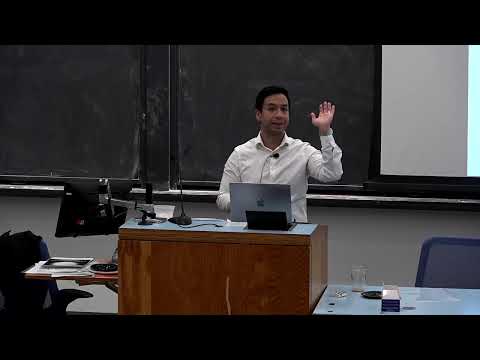
0:10 All right, I think we'll uh go ahead and get started. So, as a reminder uh in the in the last lecture, we discussed two applications of the the base filter. Uh so the base filter is this kind of basic really fundamental uh method uh for filtering, for state estimation, any kind of like probabilistic inference. uh and in the last lecture we saw two applications. So the first one is what's known as the calman filter uh which is an exact implementation of the base filter. Exact in the sense that there's no approximation. Uh but it comes at a cost which is that you need to make some really strong assumptions on the dynamics model uh and on the the sensor model. So the dynamics model needs to be linear plus Gaussian. The sensor model also needs to be linear and Gaussian. And the initial belief that you start
0:57 off with also needs to be a Gaussian. Uh and then yeah I guess under those assumptions the main result behind the common filter is that when you apply the base filter under these assumptions the belief that you end up with at every time step remains a Gaussian. Uh and then the second application that we discussed the second instantiation of the maze filter is what's known as the the particle filter where we don't make these restrictive assumptions. So we don't assume linear Gaussian uh dynamics model or sensor model. Uh but it comes at the cost of approximation error. So we don't get to represent the full kind of multimodal belief distribution that you might have. uh we approximate that with a finite set of particles that get updated at every time step based on the
1:45 probabilistic knowledge of the dynamics uh and the probabilistic sensor model as
This is the start of the transcript. Save this video free for the whole transcript, searchable and time-coded.
In this course
Related notes
Summary, takeaways, and chapters were generated by AI from the video's transcript and may contain errors. The video belongs to its creator, Introduction to Robotics @ Princeton.