Lecture 5c / 6a

Overview

The lecture completes classification evaluation by showing how decision thresholds trade precision against recall, how ROC/AUC summarizes performance across thresholds, and how class imbalance calls for balanced metrics, class-weighted training, and stratified cross-validation. It then introduces gradient-based optimization for logistic regression, defining gradient geometry and deriving gradients for an exponential model, with NumPy vectorization used to implement the cost and derivatives efficiently.

Key takeaways

For a fixed trained binary classifier, selecting a probability threshold lets a designer satisfy a required precision or recall and maximize the other metric, rather than retraining the model.
ROC AUC evaluates score ranking across all thresholds: random guessing yields 0.5, a perfect classifier yields 1, and probabilities rather than hard labels are needed to compute it.
When class prevalence is 99% versus 1%, a majority-class-only predictor can achieve 99% accuracy while completely failing the minority class, so balanced accuracy or precision-recall AUC can be more informative.
Class imbalance affects model fitting as well as evaluation; `class_weight='balanced'` reweights training examples, and stratified K-fold maintains class proportions across validation folds.
A zero gradient is only a stationary-point condition: it can indicate a minimum, maximum, or saddle point, and gradients may fail to exist at L1 regularization's sharp corner.
For the exponential prediction model `a exp(-b x_i)`, compute shared exponential terms once and use NumPy vectorization to efficiently obtain the residual cost and parameter gradients.

Chapters

0:00 Multiclass Logistic Regression and Classification Metrics Recap

One-versus-rest combines binary classifiers, while softmax models class probabilities jointly across all classes.
Softmax training minimizes cross-entropy, commonly with L1 or L2 regularization.
Accuracy treats false positives and false negatives equally, while precision and recall distinguish error tradeoffs; scikit-learn can score accuracy, precision, recall, and F1.

3:25 Probability Thresholds Trade Precision Against Recall

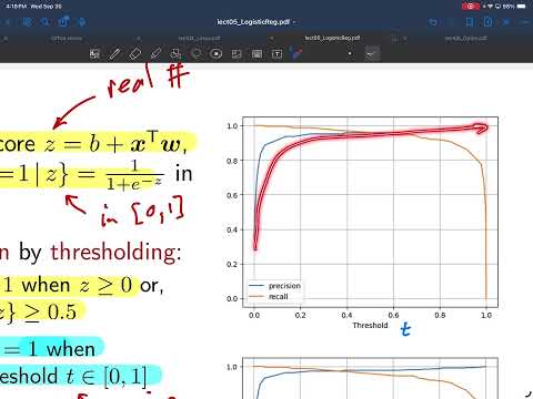
A binary classifier maps its real-valued score through a sigmoid to a probability, then predicts class 1 when the probability meets threshold t.
The conventional threshold t = 0.5 is appropriate when maximizing accuracy under equal error costs.
Increasing t generally raises precision while lowering recall; after training, choose t to meet a required precision or recall and maximize the other for the fixed classifier.

9:55 ROC Curves and AUC Compare Classifiers Across Thresholds

Sensitivity, or true positive rate, equals recall; specificity moves in the opposite direction as the decision threshold changes.
An ROC curve plots false positive rate against true positive rate across thresholds; t = 0 predicts every sample positive, while t = 1 predicts every sample negative.
Random guessing gives the diagonal ROC and AUC of 0.5, while a perfect classifier has AUC 1; an AUC below 0.5 can be improved by reversing predictions.
In scikit-learn, calculate ROC/AUC from probability scores such as `predict_proba`, not from already-thresholded hard predictions.

19:20 Multiclass Confusion Matrices and Precision Averaging

A K-class confusion matrix has K true-label rows and K predicted-label columns; diagonal entries are correct predictions and off-diagonal entries represent error types.
Row-normalizing estimates the conditional probabilities of predicted classes given each true class, making diagonal values per-class accuracies.
Overall accuracy is a prevalence-weighted average of per-class accuracy, with each class weighted by how often it occurs.
Multiclass precision and recall can be computed one-versus-rest, then combined using macro, micro, or class-frequency-weighted averaging.

25:25 Class Imbalance Requires Better Metrics and Training Practices

With 99% healthy and 1% COVID-positive cases, a classifier that predicts everyone healthy earns 99% accuracy while detecting no positive cases.
Balanced accuracy assigns each of K classes weight 1/K, exposing poor minority-class performance that overall accuracy can hide.
Precision-recall AUC is another useful evaluation option when positive examples are rare.
In scikit-learn, `class_weight='balanced'` increases the training influence of minority-class samples, while stratified K-fold preserves class proportions in every fold.

32:22 Logistic Regression Training as Cost Minimization

Binary logistic regression chooses weights W to minimize summed cross-entropy, with each sample contributing `log(1 + exp(z_i)) - y_i z_i` for labels coded 0 and 1.
The bias is incorporated as coefficient W0, so the intercept and feature weights form one parameter vector.
Scikit-learn can fit the model computationally, but understanding the optimization algorithm prepares students for training neural networks.

35:52 Gradient Direction, Stationary Points, and Differentiability

The gradient of cost J points in the direction of greatest increase and its magnitude indicates local steepness.
On a contour plot over W1 and W2, gradient arrows point uphill; zero gradient can mark a minimum, maximum, or saddle point.
Setting the gradient to zero identifies candidates rather than guaranteeing a minimum, although quadratic RSS costs have a single minimizing stationary point in the discussed setting.
L1 regularization has a nondifferentiable notch at the origin, so ordinary gradient-based methods may require more advanced alternatives.

42:22 Gradient Shapes Follow the Parameter Shapes

For a scalar cost J and a D-dimensional parameter vector W, the gradient is a D-dimensional column vector of partial derivatives.
Each partial derivative depends on the full parameter vector even though it measures change with respect to one coefficient.
When parameters form a matrix, as in multi-target regression or multinomial logistic regression, the gradient has the same matrix dimensions; higher-dimensional parameters produce tensor-shaped gradients.

45:10 Deriving Gradients for an Exponential Regression Model

The example minimizes half the residual sum of squares for predictions `y_hat_i = a exp(-b x_i)`, using parameters a and b.
The derivative with respect to a applies the chain rule to each squared residual and sums contributions across all samples.
The derivative with respect to b applies the exponential chain rule and includes the feature value x_i; the factor of one-half cancels the square's factor of two.
Stacking the two scalar partial derivatives forms the gradient vector, which changes as a and b change.

52:25 NumPy Vectorization Implements Cost and Gradients Efficiently

The Python function unpacks the parameter vector into a and b, then computes `exp(-b x_i)` once for reuse in predictions and derivatives.
It forms residuals, calculates cost as `0.5 * sum(residual**2)`, and sums vectorized expressions for both gradient entries.
NumPy elementwise operations and broadcasting avoid slow Python loops; the lecture notes that vectorization can be 10 to 100 times faster for these operations.

56:45 Midterm Scope and Study Materials

The midterm is scheduled for Friday and covers material through Unit 4, including maximum likelihood and feature selection.
Classification is excluded from the exam, no personal note sheets are allowed, and students receive the note sheet used with the practice exam.

Summary, takeaways, and chapters were generated by AI from the video's transcript and may contain errors. The video belongs to its creator, Prof. Schniter.